Conformal Geometric Algebra in Stochastic Optimization Problems ...
Conformal Geometric Algebra in Stochastic Optimization Problems ...
Conformal Geometric Algebra in Stochastic Optimization Problems ...

Create successful ePaper yourself
Turn your PDF publications into a flip-book with our unique Google optimized e-Paper software.
200 CHAPTER 7. APPLICATIONS IN COMPUTER VISION<br />
Multiple synthetic experiments are conducted: <strong>in</strong> the beg<strong>in</strong>n<strong>in</strong>g, a cloud of N<br />
Gaussian distributed po<strong>in</strong>ts {�x ′ 1...N } with a standard deviation of √ 2 and a bias<br />
of (7, 0, 0) is generated directly <strong>in</strong> front of the camera. Given the ground truth<br />
motor, denoted by M0, these po<strong>in</strong>ts are displaced yield<strong>in</strong>g the po<strong>in</strong>ts {a1...N } :=<br />
MK({�x ′ 1...N }) � M, which are <strong>in</strong>tended to represent the object model. A set of N<br />
3 × 3-covariance matrices {Σr1r1 , Σr2r2 , . . ., ΣrNrN } is generated at random so as to<br />
account for image noise. None of those <strong>in</strong>troduces an uncerta<strong>in</strong>ty parallel to the<br />
optical axis (the uncerta<strong>in</strong>ty that is to be attributed to the image po<strong>in</strong>ts is always<br />
bounded to the image plane).<br />
For each experimental run the follow<strong>in</strong>g procedure applied: for each �x ′ i<br />
, 1 ≤ i ≤<br />
N, the correspond<strong>in</strong>g Σriri is used to generate a Gaussian distributed error vector<br />
�ri ∈ �3 , which is <strong>in</strong> turn used to translate �x ′ i so as to obta<strong>in</strong> the (noisy) po<strong>in</strong>t<br />
xi = K(�x ′ i + �ri). The associated covariance matrix Σxixi is evaluated by means of<br />
the elucidations <strong>in</strong> section 6.2.1. Next the projection rays {B1...N } pass<strong>in</strong>g through<br />
the 3D-po<strong>in</strong>t cloud {x1...N } are calculated5 via Bi = (e ∧ eo ∧ xi)I, where error<br />
propagation must aga<strong>in</strong> be obeyed when evaluat<strong>in</strong>g the covariance matrices {Σb1b1 ,<br />
Σb2b2 , . .., ΣbNbN } ⊂ �6×6 . Hence the best motor � M is estimated, which fits the<br />
{a 1...N } to the correspond<strong>in</strong>g uncerta<strong>in</strong> {B 1...N }. Notice that the ground truth<br />
motor M0 is not necessarily the optimal solution for a s<strong>in</strong>gle run.<br />
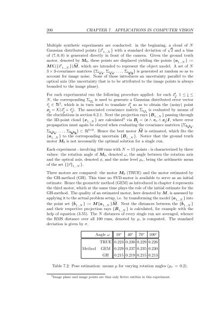
Each experiment - <strong>in</strong>volv<strong>in</strong>g 100 runs with N = 15 po<strong>in</strong>ts - is characterized by three<br />
values: the rotation angle of M0, denoted ω, the angle between the rotation axis<br />
and the optical axis, denoted φ, and the noise level µr, be<strong>in</strong>g the arithmetic mean<br />
of the set {��r� 1...N }.<br />
Three motors are compared: the motor M0 (TRUE) and the motor estimated by<br />
the GH-method (GH). This time no SVD-motor is available to serve as an <strong>in</strong>itial<br />
estimate. Hence the geometric method (GEM) as <strong>in</strong>troduced <strong>in</strong> chapter 4 represents<br />
the third motor, which at the same time plays the role of the <strong>in</strong>itial estimate for the<br />
GH-method. The quality of an estimated motor, here denoted by M, is assessed by<br />
apply<strong>in</strong>g it to the actual problem setup, i.e. by transform<strong>in</strong>g the model {a 1...N } <strong>in</strong>to<br />
the po<strong>in</strong>t set { ˆ b 1...N } := M{a 1...N } � M. Next the distances between the { ˆ b 1...N }<br />
and their respective projection rays {B 1...N } is calculated, for example with the<br />
help of equation (3.55). The N distances of every s<strong>in</strong>gle run are averaged, whence<br />
the RMS distance over all 100 runs, denoted by µ, is computed. The standard<br />
deviation is given by σ.<br />
Angle ω 10 ◦ 40 ◦ 70 ◦ 100 ◦<br />
TRUE 0.223 0.230 0.229 0.226<br />
Method GEM 0.229 0.237 0.235 0.230<br />
GH 0.215 0.219 0.215 0.213<br />
Table 7.2: Pose estimation: means µ for vary<strong>in</strong>g rotation angles (µr = 0.2).<br />
5 Image plane and image po<strong>in</strong>ts are thus only fictive entities <strong>in</strong> this experiment.