Conformal Geometric Algebra in Stochastic Optimization Problems ...

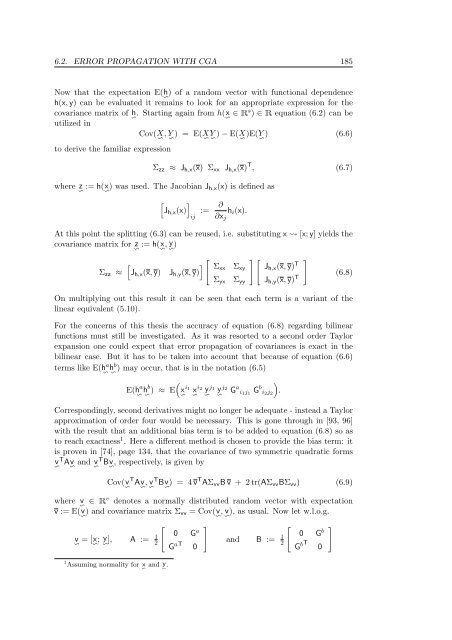
6.2. ERROR PROPAGATION WITH CGA 185
Now that the expectation E(h ∽ ) of a random vector with functional dependence
h(x,y) can be evaluated it remains to look for an appropriate expression for the
covariance matrix of h ∽ . Starting again from h(x ∽ ∈ � s ) ∈ � equation (6.2) can be
utilized in
Cov(X ∽ , Y ∽ ) = E(X ∽ Y ∽ ) − E(X ∽ )E(Y ∽ ) (6.6)
to derive the familiar expression
Σzz ≈ Jh,x(x) Σxx Jh,x(x) T , (6.7)
where z ∽ := h(x ∽ ) was used. The Jacobian Jh,x(x) is defined as
� �
Jh,x(x)
ij
:= ∂
hi(x).
∂xj
At this point the splitting (6.3) can be reused, i.e. substituting x � [x;y] yields the
covariance matrix for z ∽ := h(x ∽ , y ∽ )
Σzz ≈
�
�
Jh,x(x, y) Jh,y(x, y)
� Σxx Σxy
Σyx Σyy
�� Jh,x(x, y) T
Jh,y(x, y) T
�
(6.8)
On multiplying out this result it can be seen that each term is a variant of the
linear equivalent (5.10).
For the concerns of this thesis the accuracy of equation (6.8) regarding bilinear
functions must still be investigated. As it was resorted to a second order Taylor
expansion one could expect that error propagation of covariances is exact in the
bilinear case. But it has to be taken into account that because of equation (6.6)
terms like E(ha ) may occur, that is in the notation (6.5)
∽ hb
∽
E(h a
∽ hb
∽
�
) ≈ E x
∽
i1 i2 x∽ yj1 yj2 a
G i1j1 ∽ ∽
Gbi2j2 Correspondingly, second derivatives might no longer be adequate - instead a Taylor
approximation of order four would be necessary. This is gone through in [93, 96]
with the result that an additional bias term is to be added to equation (6.8) so as
to reach exactness1 . Here a different method is chosen to provide the bias term: it
is proven in [74], page 134, that the covariance of two symmetric quadratic forms
vTAv∽
and vTBv∽ , respectively, is given by
∽ ∽
T T
Cov(v Av∽ , v Bv∽ ) = 4v
∽ ∽
T AΣvvBv + 2tr(AΣvvBΣvv) (6.9)
where v ∽ ∈ � v denotes a normally distributed random vector with expectation
v := E(v ∽ ) and covariance matrix Σvv = Cov(v ∽ , v ∽ ), as usual. Now let w.l.o.g.
v
∽ = [x ∽ ; y], A :=
∽ 1
2
1 Assuming normality for x∽ and y ∽ .
� 0 G a
G aT
0
�
�
.
and B := 1
2
� 0 G b
G bT
0
�