Mileage-Based User Fee Winners and Losers - RAND Corporation

CHILDREN AND FAMILIES
EDUCATION AND THE ARTS
ENERGY AND ENVIRONMENT
HEALTH AND HEALTH CARE
INFRASTRUCTURE AND
TRANSPORTATION
INTERNATIONAL AFFAIRS
LAW AND BUSINESS
NATIONAL SECURITY
POPULATION AND AGING
PUBLIC SAFETY
SCIENCE AND TECHNOLOGY
TERRORISM AND
HOMELAND SECURITY
The RAND Corporation is a nonprofit institution that helps improve policy and
decisionmaking through research and analysis.
This electronic document was made available from www.rand.org as a public service
of the RAND Corporation.
Skip all front matter: Jump to Page 16
Support RAND
Browse Reports & Bookstore
Make a charitable contribution
For More Information
Visit RAND at www.rand.org
Explore the Pardee RAND Graduate School
View document details
Limited Electronic Distribution Rights
This document and trademark(s) contained herein are protected by law as indicated in a notice appearing
later in this work. This electronic representation of RAND intellectual property is provided for noncommercial
use only. Unauthorized posting of RAND electronic documents to a non-RAND website is
prohibited. RAND electronic documents are protected under copyright law. Permission is required from
RAND to reproduce, or reuse in another form, any of our research documents for commercial use. For
information on reprint and linking permissions, please see RAND Permissions.

This product is part of the Pardee RAND Graduate School (PRGS) dissertation series.
PRGS dissertations are produced by graduate fellows of the Pardee RAND Graduate
School, the world’s leading producer of Ph.D.’s in policy analysis. The dissertation has
been supervised, reviewed, and approved by the graduate fellow’s faculty committee.

Mileage-Based User Fee
Winners and Losers
An Analysis of the Distributional
Implications of Taxing Vehicle
Miles Traveled, With Projections,
2010–2030
Brian A. Weatherford
This document was submitted as a dissertation in March 2012 in partial fulfillment
of the requirements of the doctoral degree in public policy analysis at the Pardee
RAND Graduate School. The faculty committee that supervised and approved the
dissertation consisted of Martin Wachs (Chair), Howard Shatz, and Thomas Light.
Financial support for this research was generously provided by the Pardee RAND
Graduate School Energy and Environment Advisory Council. Additional financial
support was received from the Bradley Foundation and the Federal Highway
Administration.
PARDEE RAND GRADUATE SCHOOL

The Pardee RAND Graduate School dissertation series reproduces dissertations that
have been approved by the student’s dissertation committee.
The RAND Corporation is a nonprofit institution that helps improve policy and
decisionmaking through research and analysis. RAND’s publications do not necessarily
reflect the opinions of its research clients and sponsors.
R ® is a registered trademark.
All rights reserved. No part of this book may be reproduced in any form by any
electronic or mechanical means (including photocopying, recording, or information
storage and retrieval) without permission in writing from RAND.
Published 2012 by the RAND Corporation
1776 Main Street, P.O. Box 2138, Santa Monica, CA 90407-2138
1200 South Hayes Street, Arlington, VA 22202-5050
4570 Fifth Avenue, Suite 600, Pittsburgh, PA 15213-2665
RAND URL: http://www.rand.org
To order RAND documents or to obtain additional information, contact
Distribution Services: Telephone: (310) 451-7002;
Fax: (310) 451-6915; Email: order@rand.org

ABSTRACT
The mileage-based user fee (MBUF) is a leading alternative to the gasoline tax. Instead of
taxing gasoline consumption, the MBUF would directly tax drivers based on their vehicle miles
traveled (VMT). Equity is a commonly raised public acceptance concern regarding MBUFs. This
study uses household-level survey data of travel behavior and vehicle ownership from the 2001 and
the 2009 National Household Travel Survey (NHTS) to estimate changes in annual household
demand for VMT in response to changes in the cost of driving that result from adopting MBUF
alternatives. Distributional implications are estimated for an equivalent flat-rate MBUF, an increased
fuel tax rate and it’s equivalent flat-rate MBUF, and three alternative MBUF rate structures: a 1 cent
MBUF added to the current fuel tax, a tiered rate MBUF based on vehicle fuel economy, and a much
increased MBUF rate. The distributional implications are then projected over the years 2015 - 2030
under eight different macroeconomic and policy scenarios.
The research finds that a flat-rate MBUF would be no more or less regressive than fuel taxes,
now or in the future. An increase in the tax rate, whether an MBUF or a fuel tax, causes
transportation revenue collection to become less regressive because low income households have a
more elastic response to changes in price than middle and high income households. MBUF
“winners” include retired households and households located in rural areas. On average, an MBUF
would reduce the tax burdens of these groups. MBUF “losers” are households in urban and
suburban areas. The projections suggest that the distributional implications of MBUFs are unlikely
to change in future years. Changes in the cost of driving, either from a higher tax rate, or other
factors, appears to have a greater impact on the equity of transportation finance than whether the
tax is collected by the gallon or by the mile. These results are robust to alternative sources of data
and model assumptions.
The findings are significant because they suggest that equity considerations based on ability
to pay will not be a significant reason to oppose or support the adoption of MBUFs. While the
equity implications of MBUFs are minimal, however, some groups, especially rural states, may find
that the potential equity benefits of MBUFs could be overwhelmed by an increase in the tax rate to
cover the higher costs of collecting and administering them. Concerns about the impacts of flat-rate
MBUFs on vehicle fuel efficiency and greenhouse gas emissions are valid but, at current oil prices,
the tax rate is a small percentage of the total cost of gasoline. Therefore, the overall price signals still
encourage fuel efficiency. Regardless, it is possible to structure an MBUF that provides incentives for
fuel efficiency while maintaining other favorable qualities of MBUFs such as their economic
efficiency and fiscal sustainability.
Page 5 of 131

ACKNOWLEDGEMENTS
I would like to acknowledge the support, guidance and intellectual contributions of the three
members of my dissertation committee. Professor Martin Wachs chaired my dissertation committee.
Marty has a reputation in the transportation studies community for being an extraordinary graduate
student advisor. The reputation is well deserved. Marty has been generous in sharing his time and
his vast professional experience with me. Howard Shatz was the very first member of my
dissertation committee. Years before I selected a topic, I knew that I wanted to work with Howard
and I greatly appreciate his patience, generosity, and encouragement as I considered, and rejected,
various topics over a period of nearly seven years. Howard is brilliant and we share many intellectual
pursuits, but, most importantly, Howard is a kind man and dedicated to his graduate students. The
third member of my dissertation committee is Thomas Light. Tom was a natural addition because
of our shared passion for the discipline of transportation economics. While I appreciate our
friendship, I would like to acknowledge the great deal of time and attention that Tom paid to my
work on this dissertation. My outside reader is Professor Mark Burris of Texas A&M University. His
insightful comments and critiques directly and indirectly led to a much strengthened final product.
Mark was very thorough in his review and responded very quickly. The contributions of these four
scholars were invaluable to the completion of this dissertation.
I would like to also acknowledge the financial support of the Pardee RAND Graduate
School Energy and Environment Advisory Council. This group was assembled by the previous
Dean of the RAND Graduate School, John Graham. I was very fortunate to receive two
consecutive fellowships to fund my final two years of research and writing. As a practical matter, I
may not have been able to complete this dissertation without the financial support of this group. I
would also like to acknowledge Dean Graham’s interest in my research and his critiques of my
assumptions regarding American travel. His influences are strongly felt in this dissertation. I would
like to further acknowledge the Bradley Foundation for their financial support as I worked to
identify a dissertation topic. This support was fully the result of the work of Professor Richard Neu.
I appreciate his early guidance and regret somewhat that we were unable to scope a dissertation
topic in the discipline of economic geography. I also acknowledge the financial support of the
Federal Highway Administration which funded some of my research travel.
The past seven years studying and working at the RAND Corporation were wonderful and
transformative. As a research institution, this is entirely due to the qualities of the people who
taught, advised, counseled, supervised, and supported me. I am choosing not to name them all
because I am terrified that I will inadvertently exclude a mentor or a dear friend. I would like to
acknowledge several individuals, however, who made particularly important contributions to the
dissertation and the completion of my degree. My colleague Paul Sorensen has also been researching
MBUFs and I frequently called on him to discuss the topic. My classmate Sarah Outcault held me
accountable to my daily goals and without her dedication to our partnership, as well as her constant
support and encouragement, I am not sure I would have completed my dissertation pre-prospectus.
The RAND library staff, especially Roberta Shanman, provided invaluable research and technical
assistance to me. While all of the staff at the RAND Graduate School are wonderful and helpful, I
would like to especially acknowledge Assistant Dean Rachel Swanger. Rachel has an incredibly
difficult job and I frankly have no idea how she manages to accomplish everything that she does. My
time at the RAND graduate school has been entirely a period of transition from one administration
to the next; Rachel was the only constant. Her dedication to the school is unparalleled with the
notable exception of Founding Dean, Charlie Wolf. I want to acknowledge and express admiration
for Professor Wolf ’s continued and lasting contributions to the graduate school.
Page 7 of 131

Lastly, I would especially like to acknowledge the enduring patience and support of my wife,
Tina, and our children, Achilles and Vincent. Without their presence in my life, I might have written
a dissertation in fewer years, but those years would have been remarkably empty. And, so, this is
dedicated to my family: may all our years be full and worthwhile.
Page 8 of 131

CONTENTS
Glossary ............................................................................................................................................. 11
1. Mileage-Based User Fees .......................................................................................................... 13
Motor Fuel Taxes are Not a Viable Long-Term Source of Transportation Revenue ..... 13
Moving Towards a Tax on Vehicle Miles Traveled ............................................................... 17
The Equity Implications of MBUFs Are Uncertain ............................................................ 19
2. The Equity of Highway User Fees and Taxes ....................................................................... 21
Externalities and Pigouvian Taxes ........................................................................................... 21
Prior findings Regarding the Equity of Fuel taxes and Road Pricing ................................ 22
Geographical and Jurisdictional Equity of Transportation Finance .................................. 23
Contribution of Research to Policy and to Knowledge ....................................................... 23
3. Data and Model ......................................................................................................................... 25
Data .............................................................................................................................................. 25
Model ........................................................................................................................................... 28
4. Methodology .............................................................................................................................. 43
Overview ..................................................................................................................................... 43
Distributional Analysis of Alternatives .................................................................................. 43
Projections .................................................................................................................................. 59
5. The Equity Effects of Mileage-Based User Fees ................................................................. 63
Key Findings ............................................................................................................................... 63
Flat-Rate MBUFs Are No More or Less Regressive Than Fuel Taxes .............................. 64
MBUF Winners and Losers ...................................................................................................... 71
Increased Rates and Alternative Rate Structures .................................................................. 73
Jurisdictional or Political Equity .............................................................................................. 80
Sensitivity Analysis ..................................................................................................................... 83
Page 9 of 131

6. Future Distributional Implications, 2010 - 2030 ................................................................... 91
Key Findings ............................................................................................................................... 91
MBUFs Provide Revenue Sustainability ................................................................................. 91
No Change in MBUF Distributional Implications ............................................................... 93
Fuel Price and Fuel Economy Matter More than Tax Rate ................................................ 97
7. Conclusion .................................................................................................................................. 99
Discussion of Findings ............................................................................................................. 99
Contributions to Knowledge ................................................................................................. 100
Limitations and Opportunities for Further Research ......................................................... 100
Policy Considerations .............................................................................................................. 101
A. Technical Appendix ................................................................................................................. 105
Data Cleaning ........................................................................................................................... 105
Construction of Key Variables .............................................................................................. 108
Calcualting the Suits Index ..................................................................................................... 112
Calculating the Change in Consumer Surplus ..................................................................... 114
Calculating the Net Change in Household Welfare ............................................................ 115
B. Additional Tables ..................................................................................................................... 117
List of References .......................................................................................................................... 127
Page 10 of 131

GLOSSARY
Symbol
Definition
AAA
American Automobile Association
AEO
Annual Energy Outlook
BLS
Bureau of Labor Statistics
CAFE
Corporate Average Fuel Economy
CBO
Congressional Budget Office
CPI
consumer price index
EIA
Energy Information Administration
EPA
Environmental Protection Agency
EV
electric vehicle
FHWA
Federal Highway Administration
GAO
Government Accountability Office
GHG
greenhouse gas
GPM gallons per mile, GPM = MPG -1
HEV
hybrid-electric vehicle
HTF
Highway Trust Fund
MBUF
mileage-based user fee
MPG miles per gallon, GPM = MPG -1
NHTS
National Household Travel Survey
NHTSA
National Highway Traffic Safety Administration
OECD
Organization for Economic Co-operation and Development
ORNL
Oak Ridge National Laboratory
PHEV
plug-in hybrid electric vehicle
PRGS
Pardee RAND Graduate School
RV
recreational vehicle (motor home)
SAFETEA–LU Safe, Accountable, Flexible, Efficient Transportation Equity Act: A
Legacy for Users
SUV
sport utility vehicle
TRB
Transportation Research Board of the National Academies
VMT
vehicle-miles traveled
Page 11 of 131

1. MILEAGE-BASED USER FEES
MOTOR FUEL TAXES ARE NOT A VIABLE LONG-TERM SOURCE OF
TRANSPORTATION REVENUE
Roads in the United States are generally provided by the public sector and funded using
public revenue. Gasoline and diesel fuel taxes provide a third of all public revenues that are used to
operate, maintain and expand the surface transportation system in the United States. 1 A diversity of
general fund sources and user fees comprise the remaining amount. As the largest single source of
highway revenue, there is considerable public interest in understanding the efficiency, equity, and the
long-term viability of fuel taxes (Committee for the Study of the Long-Term Viability of Fuel Taxes
for Transportation Finance 2006; Congressional Budget Office 2011).
The motor fuel tax is constantly under pressure from two sources: increasing construction
costs and increasing vehicle fuel efficiency. Throughout the history of the fuel tax, legislators have
had difficulty routinely increasing the gasoline and diesel fuel tax rates so that total fuel tax revenue
keeps pace with funding needs. 2 The costs of constructing and maintaining roads have grown
rapidly, more rapidly, by some accounts, than the overall consumer price index (CPI) and certainly
faster than the federal gasoline tax rate (Luo 2011). The federal gasoline tax was last increased in
1993 and, since then, the CPI has advanced by 51 percent and the California Construction Cost
Index has advanced by 82 percent. 3
At the same time, total fuel tax receipts fail to keep pace with the amount of travel. As
vehicle fuel economy improves, the amount of tax collected for each mile traveled declines. As total
vehicle miles traveled (VMT) increases, there is an increased need for highway maintenance and to
expand the capacity of existing roads and transit systems. Vehicle fuel efficiency, which is typically
measured in miles per gallon (MPG), dramatically improved during the 1980s following an increase
in fuel prices and the adoption of the Corporate Average Fuel Economy (CAFE) standards in 1975
(National Highway Transportation Safety Administration 2011). Further improvements to vehicle
fuel economy slowed during the late 1990’s and yearly 2000’s as the initial CAFE standards were
completely phased in and gasoline prices reached historic lows. 4 Vehicle fuel efficiency is, however,
once again improving rapidly. Gasoline prices increased by 134 percent, from $1.75 per gallon in July
2002 to just over $4.00 in July 2008, and consumers are responding by purchasing more fuel efficient
cars. Sales of highly fuel efficient hybrid electric vehicles (HEV), in particular, are growing faster
than the overall automobile market (CBSNews July 6, 2009).
1 This includes transit and excludes private infrastructure. In 2008, federal, state, and local fuel taxes generated approximately $78
billion in revenue; total highway and transit revenue across all levels of government was $235 billion (FHWA, 2010; Federal Transit
Administration, 2010). For comparison, private railroads generated $61.2 billion in operating revenue in 2008 (Association of
American Railroads, 2010).
2 The federal gasoline tax rate is 18.4 cents per gallon of gasoline and 24.4 cents per gallon of diesel. All states levy a per-gallon excise
tax and many also impose an ad valorem sales tax. In addition, many states allow local governments to levy a local option excise or
sales tax on gasoline. In January 2011, total taxes on gasoline ranged from 20.4 cents per gallon in Alaska to 66.1 cents per gallon in
California; the volume-weighted national average was 48.1 cents per gallon of gasoline and 53.1 cents per gallon of diesel (American
Petroleum Institute, 2011).
3 Highway construction costs are more volatile than the CPI and are subject to competition from construction in other sectors and
from global competition for steel, cement, and other commodities. For example, construction costs tracked by the California
Department of Transportation fell sharply between 2006 and 2010. This index, where 2007 = 100, was 42.2 in 1993, 104.1 in 2006,
95 in 2008, 78.4 in 2009 and 76.8 in 2010. The percent change 1993-2010 is 82 percent.
4 Gasoline prices reached a historic low in February 1999 with an average nominal price (all formulations, including taxes) of $0.96 per
gallon equivalent to $1.27 in real 2010 dollars (US Energy Information Administration 2011).
Page 13 of 131

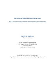
The result is that the real value of the fuel tax is steadily declining. While some states, such as
Maine and Wisconsin, regularly adjust their fuel tax rates, federal fuel tax rates were last increased in
1993 (Ang-Olson, Wachs, and Taylor 2000; Federal Highway Administration 2010). Since then, as
illustrated in Figure 1.1, the real value of the federal gasoline tax has declined by 42 percent. Without
an immediate increase in the fuel tax rate, an unlikely event, this trend will accelerate over the
coming years. Several sets of increasingly stringent CAFE regulations, currently applying to new
light duty vehicles through model year 2016 and heavy duty vehicles though model year 2018, have
been adopted by the Environmental Protection Agency (EPA) and the National Highway
Transportation Safety Administration (NHTSA) since 2006 (US NHTSA 2011). The Energy
Information Administration (EIA) projects that, given current policy and technology, the fuel
efficiency of the overall vehicle population will improve by 25 percent between 2010 and 2030 (US
EIA 2011a). This will cause the average fuel tax rate (per mile) to fall proportionately, prior to
accounting for deleterious effects of inflation. Additional mandates to improve vehicle fuel
efficiency, along with further technical advances to enable those reductions, are obviously possible,
if not highly likely.
Figure 1.1: Federal Gasoline Tax Rate, Real Cents per Mile Traveled, 1970 - 2010
1.8
1.6
1.4
2010 Cents Per Mile
1.2
1.0
0.8
0.6
0.4
0.2
0.0
1970 1975 1980 1985 1990 1995 2000 2005 2010
Year
Note: The real tax rate is calculated using the CPI. Alternatively, it is possible to use a construction cost index, such as
the previously described California Construction Cost Index, which might more accurately reflect the real value of the
tax rate with respect to constructing transportation projects. However, the volatility of construction commodity prices
could mask the underlying historical trends of increasing prices overall and increasing average vehicle fuel economy.
Therefore, all dollar values in the dissertation, unless otherwise noted, are in 2010 dollars, after adjusting for inflation
using the CPI (all urban consumers, all items, not seasonally adjusted, series id# CUUR0000SA0).
Sources: Federal Highway Administration (FHWA), Highways Statistics Series, 1995-2009, Tables FE-101A, VM-201A and
VM-1.
Page 14 of 131

Additionally, fully electric vehicles (EV) and plug-in hybrid-electric vehicles (PHEV) are now
being sold to consumers by major automobile manufacturers. While there are currently a small
number of electric vehicles on the road, the market for this technology is poised to grow rapidly and
could account for 5-15 percent of the automobile market by 2020 (Bedi et al. 2011). Estimates for
sales volumes of EV and PHEV automobiles vary and are highly speculative but nonetheless
stimulate further concern about the long-term viability of gasoline taxes because these vehicles pay
little to no tax (Ang-Olson, Wachs, and Taylor 2000; Dignan 2010; Eisenstein 2010; Hajiamiri 2010).
The real value of the fuel tax, relative to funding needs, will continue to decline as construction
costs rise, vehicle fuel economy continues to improve and the number of EVs sold increases. It is
unclear whether federal gasoline and diesel taxes will be able to generate sufficient revenue to
maintain and improve the nation’s surface transportation network in future years.
Three separate commissions were formed between 2003 and 2009 to review national
transportation finance needs and sources of revenue. The earliest, the Committee for the Study of
the Long-Term Viability of Fuel Taxes for Transportation Finance, was convened by the
Transportation Research Board of the National Academies (TRB). 5 This committee met between
2003 and 2005 to consider the challenges and the benefits of the gasoline tax against the likely
opportunities and obstacles of alternative sources of revenue (Committee for the Study of the
Long-Term Viability of Fuel Taxes for Transportation Finance 2006). The committee concluded
that fuel taxes would be viable over the next two decades but reform was necessary. Specifically, this
committee recommended that fuel taxes should be maintained and increased in the short-term. The
public sector should also begin to transition towards charging highway users directly based on the
number of miles traveled, instead of on fuel consumption. The committee expressed support for
expanded use of toll roads and toll lanes on free highways to better manage congestion and to
generate some additional revenue. However, the committee endorsed taxes on miles traveled as “the
most promising technique for directly assessing road users for the costs of individual trips within a
comprehensive fee scheme that will generate revenue to cover the costs of the highway program”
(Committee for the Study of the Long-Term Viability of Fuel Taxes for Transportation Finance
2006, 4).
The 2005 federal transportation authorization bill, the Safe, Accountable, Flexible, and
Efficient Transportation Equity Act: A Legacy for Users (SAFETEA–LU), created two separate
commissions with similar mandates; both would assess current revenues and possible alternatives
and make recommendations to Congress. Section 1909 of SAFETEA–LU established the National
Surface Transportation Policy and Revenue Study Commission (2007). The “Policy Commission”
consisted of 12 members. They presented their findings, which were not unanimous, to Congress in
2007. The Commission’s Chairwoman, Secretary of Transportation Mary Peters, was among three
dissenting commissioners who argued that the primary problem facing the nation’s transportation
system was not insufficient revenue but an inability to manage demand. Both the dissenting group
and the majority of the Policy Commission agreed that the use of tolling and congestion pricing be
5 The candidate’s dissertation committee chair, Professor Martin Wachs, was one of the 14 members of this committee.
Page 15 of 131

expanded and that a vehicle mileage-based user fee (MBUF) should be considered. In particular, the
dissenting group writes:
“Thanks to technology development and the leadership of a number of State and
local officials, the move toward direct pricing is underway at the State and local
level. A change from an indirect to a direct pricing system can and should ensure
continued access to transportation systems for all Americans, regardless of income.
In fact, when contrasted to the highly regressive nature of higher fuel taxes and
congestion itself, direct pricing is likely to be a far more fair system” (National
Surface Transportation Policy and Revenue Study Commission 2007, 67). 6
The majority of the Policy Commission recommended that the next transportation authorization bill
fund “a major national study to develop the specific mechanisms and strategies for transitioning to
an [MBUF] alternative to the fuel tax to fund surface transportation programs” (National Surface
Transportation Policy and Revenue Study Commission 2007, 53).
Section 11142 of SAFETEA–LU established the 15 member National Surface
Transportation Infrastructure Financing Commission (2009). The “Financing Commission”
reported their unanimous findings to Congress, the Department of Transportation, and the
Department of the Treasury in 2009. While the work of this commission overlaps considerably with
the work of the Policy Commission, the focus of their study is “on how revenues should be raised,
including whether there are other mechanisms or funds that could augment the current means for
funding and financing highway and transit infrastructure” (National Surface Transportation
Infrastructure Financing Commission 2009, 5). The Financing Commission’s findings echo the
findings and recommendations of the two prior study groups; the current system of indirectly
taxing travel by taxing users’ fuel consumption is unsustainable over the long-term and the system
must transition to direct charges on VMT (National Surface Transportation Infrastructure Financing
Commission 2009, 7-16).
It is remarkable that these three disparate groups agree on the need to replace the gasoline
tax with an MBUF despite conflicting conclusions regarding when the fuel tax will no longer be
viable, how much funding is ultimately needed, the role of the federal government in transportation
relative to the states, the types of transportation projects that should be funded by the federal
government, and how these investments should be prioritized. This reflects or, perhaps, is
motivating a growing consensus among senior transportation policy experts and advisors that
transportation will be primarily funded by direct user charges instead of gasoline taxes (Forkenbrock
and Hanley 2006; Shane et al. 2010). While there is consensus regarding the general concept and the
need for a vehicle mileage-based tax or user fee, there remains considerable disagreement about the
technical details, timeline, costs, benefits, system impacts, and social effects of MBUFs. 7
6 The term “regressive” means that the tax burden falls more heavily on low income taxpayers than on high income taxpayers relative
to their ability to pay. It is the opposite of a “progressive” tax such as the federal income tax.
7 A tax on VMT is commonly referred to as a “Mileage-Based User Fee” or a “VMT fee.” The use of the term “fee” may be a
conscious, intentional semantic choice by those advocating for the adoption of one. Following conventional usage, the term
“MBUF” will be used though out the dissertation but it is always treated as a tax. The distinction between a user fee and a tax is
important although there remains some disagreement over the intent and the precise legal definition of a “user fee.” In general, the
revenue from a tax can be used for any purpose while the revenue from a user fee may only be used to provide the public good or
service on which the fee is being charged (Gillette and Hopkins 1987). There are often further distinctions between the ease to levy
and change the rate of a tax (difficult) and a user fee (relatively easy).
Page 16 of 131

MOVING TOWARDS A TAX ON VEHICLE MILES TRAVELED
The concept of an MBUF is an appealing alternative to the gasoline tax because it could be
more economically efficient, fiscally sustainable, accurate and transparent (Parry and Small 2005;
Forkenbrock and Hanley 2006; Safirova, Houde, and Harrington 2007; Sorensen, Wachs, and Ecola
2010; Baker and Goodin 2011). These potential benefits have led to several technical feasibility
studies and trials (Forkenbrock and Kuhl 2002; Donath et al. 2003; Whitty 2007; Puget Sound
Regional Council 2008; Sorensen et al. 2009; Sorensen, Wachs, and Ecola 2010; Baker and Goodin
2011; Public Policy Center 2011; US CBO 2011). While many see the MBUF as a future alternative,
there is interest in taking immediate steps to begin transitioning away from the gasoline tax to the
MBUF (Forkenbrock 2005; Sorensen et al. 2009). Given the level of interest in the MBUF concept,
there is a growing body of research on various aspects of MBUFs spanning technical feasibility
concerns (Donath et al. 2003) to consumer perceptions (Baker and Goodin 2011). Two large-scale
MBUF technical feasibility trials have been completed; one in Oregon (Whitty 2007) and the other in
the Puget Sound metropolitan region of Washington (Puget Sound Regional Council 2008). A major
national trial is being conducted by the University of Iowa in 12 locations around the country
(Sorensen, Wachs, and Ecola 2010; Public Policy Center 2011). These trials have demonstrated the
proof of concept and have stimulated interest in funding additional trials in other states and a more
extensive national trial (National Surface Transportation Policy and Revenue Study Commission
2007; Sorensen, Wachs, and Ecola 2010).
The primary motivation for considering the adoption of an MBUF is better revenue
sustainability. Improving vehicle fuel efficiency and the growth in the consumer market for EVs and
PHEVs will continue to diminish the value of the fuel taxes (Hajiamiri 2010). While the MBUF will
not be immune from inflationary pressure, it will staunch the deleterious effects on revenue from
these forces. Further, if successfully implemented as a user fee, the MBUF may be politically easier
to adjust for changes in construction costs. An MBUF is not the only response to the falling real
value of the fuel tax. The fuel tax is supplemented in many states with local fuel taxes, state and local
sales taxes, and general funds. Shortfalls in the HTF have been supplemented with more than $30
billion in general funds since 2008 (US General Accountability Office 2010). However, an MBUF
may be preferred by some because it has economic efficiency advantages over these alternatives.
MBUFs can be more economically efficient than gasoline taxes and general fund sources for
several reasons. A flat-rate MBUF more directly reflects many of the costs of driving, including
externalities such congestion, accidents and some air pollutants. With the exception of carbon
dioxide emissions and their impact on the risk of global warming, these externalities are more
directly related to VMT than to fuel consumption (Parry, Walls, and Harrington 2007). 8 A direct tax
on VMT is also more efficient than fuel taxes because of the rebound effect. 9 There is no direct
relationship between driving and sales or income, although there is certainly an indirect correlation,
making these the least economically efficient tax mechanism.
There are various methods of metering and reporting a vehicle’s VMT for the purpose of
charging drivers an MBUF with varying degrees of accuracy, geographic resolution, technical
sophistication, cost, and burden on the user (Sorensen et al. 2009). A more technologically advanced
method could vary the mileage charge by road being travelled and by the time of day (Sorensen,
Wachs, and Ecola 2010). This has many potential benefits. Among these benefits is the potential to
8 Local air pollutants, such as carbon monoxide, nitrogen oxides, and suspended particulates are regulated by the mile.
9 The rebound effect describes how consumers respond to fuel taxes and higher gasoline prices not only reducing VMT but also by
purchasing more fuel efficient vehicles. The more efficient vehicles reduce the per-mile cost of driving and so consumers respond
by increasing VMT, partially offsetting the reduction expected from the per-gallon price increase.
Page 17 of 131

adopt a rate structure that varies by the road being traveled and by the time of day. Variable pricing
could be used to reduce traffic congestion very effectively and is the greatest source of potential
benefit to highway users (Parry, Walls, and Harrington 2007). By managing travel demand more
efficiently and effectively, investment needs could also be minimized (Small and Van Dender 2007).
Adopting a sophisticated MBUF collection system would also allow for an improved understand of
where transportation investments are most urgently needed.
An MBUF collection system that allows for accurately charging users based on exactly where
on the transportation system they have driven also allows for a more accurate spatial understanding
of travel demands. This will enable a more accurate apportionment of revenue to local jurisdictions
and prevent interstate tax evasion. 10 Currently, it is possible to know with certainty only where the
fuel was purchased and not where it is consumed. This more accurate data may also be used to
better calibrate transportation planning models which may lead to improved long-term plans
(Sorensen, Wachs, and Ecola 2010). The potentially high level of detail and accuracy of the data
raises concern for traveler privacy.
There are several concerns about MBUFs which may offset the potential benefits. One of
the first concerns expressed by members of the general public upon hearing about MBUF proposals
is privacy (Baker and Goodin 2011). The technical feasibility studies have demonstrated that user
privacy can be protected (Forkenbrock and Kuhl 2002; Whitty 2007; Sorensen, Wachs, and Ecola
2010). Nonetheless, the perception among the public that MBUF metering systems can be used by
the government to track individuals will likely persist.
Another significant problem with MBUFs is the higher cost of administering, collecting and
enforcing the tax. Fuel taxes are collected indirectly from users at central distribution points and the
total costs are about 1 percent of total revenue (Balducci et al. 2011). With no MBUF system in
operation anywhere in the world, it is not possible to accurately estimate the costs of a state or
national system at this time. The costs of accurately collecting the fee directly from every driver,
enforcing compliance, and managing disputes will undoubtedly be higher than the fuel tax. The
closest analogue to an MBUF, in operation, is a toll road. These require an average of 34 percent of
revenue to operate and collect (Balducci et al. 2011). A full scale MBUF system will likely be more
efficient than a single tolled road, but the costs will clearly be greater than under the current fuel tax.
Adopting an MBUF to support current levels of public funding of transportation will necessarily
require a higher tax rate in order to generate sufficient revenue to offset the increase in collection,
administration, and enforcement costs. Analysts have proposed that benefits from additional
services could help to partially offset the higher costs (Sorensen, Wachs, and Ecola 2010; Baker and
Goodin 2011).
Some of these other potential benefits to drivers from an advanced MBUF collection system
include “pay as you drive” (PAYD) automobile insurance, automated parking and toll payment,
location dependent travel and safety services, and media connectivity services for vehicle passengers
(Sorensen, Wachs, and Ecola 2010). While these possible benefits are promising, more research is
needed to understand whether they are actually feasible and how much drivers will value them. More
research is also needed to understand the equity implications of MBUFs, another frequently
expressed concern and potential benefit (Cambridge Systematics 2009; Taylor 2010; Baker and
Goodin 2011).
10 Interstate tax evasion is when residents of a state with a high fuel tax rate travel to another state to purchase motor fuel taxed at a
relatively lower rate. Alternative MBUF implementations will, however, introduce new and varied possibilities for tax evasion.
Page 18 of 131

THE EQUITY IMPLICATIONS OF MBUFS ARE UNCERTAIN
Charging drivers by the mile instead of by the gallon is a major policy change with uncertain
implications for the distribution of the tax burden among households. The overall equity of MBUFs
will likely be similar to that of fuel taxes because of the close relationship between total VMT and
total fuel consumption (Parry and Small 2005). Nonetheless, the distributional implications are
uncertain because the distribution of vehicle fuel economy across income levels and other groups of
households within the population may change over time. The distribution of vehicle fuel economy
determines, in part, the relative equity implications when moving from a fuel tax to an MBUF. This
distribution appears to be changing as fuel prices rise, vehicle fuel economy regulations become
increasingly stringent, and a variety of alternative fuel vehicles become commercially available. In
addition, there are other characteristics of households and groups of households that can influence
changes in distribution of the burden of a tax which are even more difficult to directly observe and
predict. With MBUF implementation far from certain and far from immediate, the uncertainty only
increases with time.
Several prior studies, all using the 2001 National Household Travel Survey, find that
replacing the fuel tax with a flat rate MBUF would reduce the taxes paid by low income and rural
households and increase the taxes paid by middle income and urban households (Zhang et al. 2009;
McMullen, Zhang, and Nakahara 2010; Weatherford 2011). These findings are consistent with other
research on the equity of the gasoline tax that shows that low income and rural households own
vehicles that are older and less fuel efficient than the overall population (West 2005; Bento et al.
2009). Households owning less fuel efficient vehicles would benefit from a flat-rate MBUF because
their current fuel tax rate per mile is higher than households that own high-MPG vehicles (Baker,
Russ, and Goodin 2011). These prior studies of the distributional implications of MBUFs all use
data from a survey, the 2001 NHTS, conducted more than a decade ago. They only consider the
equity implications from one type of flat-rate MBUF that generates the same, or approximately, the
same amount of revenue, and do not estimate how future macroeconomic conditions or future
improvements in vehicle fuel economy might affect the equity of an MBUF. Research is needed to
more fully, comprehensively, and confidently understand the equity implications of MBUFs.
This dissertation presents the methodological approach and the results of a comprehensive
policy research study of the equity implications of MBUFs. Specifically this dissertation answers the
question:
• What are the distributional implications of adopting an MBUF to replace or supplement
the gasoline tax as a future source of public revenue for maintaining and expanding the
surface transportation system?
And, to this end, it answers the following three research questions:
• Are MBUFs more or less regressive than fuel taxes?
• Who are the winners and losers of a flat-rate MBUF?
• How do alternative MBUF rates and rate structures affect the distributional implications
of MBUFs relative to fuel taxes and each other?
The results are projected over the future years 2015-2035 and under alternative future
macroeconomic conditions in order to understand how sensitive the results are to assumptions
about future changes in prices, household income, and vehicle fuel economy.
Page 19 of 131

Chapter 2 introduces specific equity concepts and reviews the findings from equity studies
of gasoline taxes and other travel related fees and charges such as toll lanes and emissions taxes.
Chapter 3 describes the data used in this study, the 2001 and 2009 NHTS. Chapter 4 describes the
methodological approach followed in this study. Chapter 5 presents and discusses the results of the
distributional implications of MBUF policy alternatives. Chapter 6 presents and discusses the results
of the projections of the distributional implications of MBUFs in years 2015-2035. Chapter 7
concludes the dissertation with a discussion of the limitations of the research, opportunities for
further research, and guidelines for considering equity in MBUF policy.
Page 20 of 131

2. THE EQUITY OF HIGHWAY USER FEES AND TAXES
Equity is a critical concern in the analysis and comparison of tax policies (Brewer and
deLeon 1983; Musgrave and Musgrave 1989; Taylor 2010). Policy makers and taxpayers are often
interested in whether a new tax will be more or less “equitable.” However, equity concepts can be
imprecisely defined and susceptible to a subjective evaluation (Levinson 2010). This dissertation
investigates the relative distributional implications of implementing MBUF taxes of various designs.
In other words, relative to the existing tax system, who will pay more tax, or less, relative to others
after adopting an MBUF? Who will benefit more, or less, relative to others from any change in tax
revenue and externalities?
The incidence of a tax describes how much of a tax is paid by producers and how much is
paid by consumers (Musgrave and Musgrave 1989). For most goods, regardless of whether the tax is
directly levied on a supplier, as is the case with fuel taxes, or a consumer, the tax burden is shared. 11
Tax burden is a phase that describes the price and income effect of a tax dollar all are impacted by
the taxis split between the two. The proportion of the tax burden paid by each party varies
depending on the structure of the market, the price elasticity of demand relative to the price
elasticity of supply, and other factors (Musgrave and Musgrave 1989). While the direct incidence of
the current gasoline tax falls on the gasoline distributor, the consumer pays all or nearly all of an
increase in the tax rate (Alm, Sennoga, and Skidmore 2009).
The most obvious difference between a fuel tax and an MBUF is the change in the party
upon which the tax is initially levied. Otherwise, as long as vehicle choice is held constant, the
societal incidence of the tax is not expected to differ from the gasoline tax since both directly affect
consumers driving behavior regarding whether or not to take a trip. 12 Instead of a higher-level
consideration of incidence, this dissertation is focused on understanding how the burden of similar
taxes varies between households and groups of households. In addition to the amount of tax paid as
a part of their costs of driving, households also bear the burden of a fuel tax or MBUF in other
ways. Were there no tax, for example, the cost of driving would be lower and so households would
make a marginal number of additional trips (McCarthy 2001). Driving also results in various
externalities such as traffic congestion and air pollution (Parry and Small 2005; West 2005). In
addition, the revenue raised by the tax does not leave the economy. As previosuly discussed in
Chapter 1, fuel tax and MBUF revenues are used to finance the maintenance and expansion of the
transportation system with socail benefits. The fiscal and social benefits of a tax can partially ofset
the economic costs imposed on society and the distribution of these benefits should be considered
when comparing tax burdens of various groups (Bento et al. 2009; Levinson 2010).
EXTERNALITIES AND PIGOUVIAN TAXES
Many taxed goods have negative externalities associated with their use or consumption.
Cigarettes, for example, produce a health risk to the individual, but also create costs for society,
including secondhand smoke and insurance and healthcare costs that are not internalized by the
individual. A Pigouvian tax adds the marginal social cost of consumption to a good with
11 A number of terms are defined in this Chapter but no effort has been made to do so rigorously and mathematically. It would be
tedious to read and duplicative of much good work that has preceded this dissertation. Many excellent references are cited for those
readers seeking further clarity.
12 As discussed later in Chapter 3, once the vehicle choice assumption is relaxed other incidence changes are possible. This effect is
relatively small (Bento et al. 2009).
Page 21 of 131

externalities in order to cause the consumer to internalize the full cost of consuming the good, and
reduce their demand to the socially optimal level (Baumol and Oates 1988).
Gasoline taxes are sometimes promoted as a Pigouvian tax to reduce fuel consumption and
the risk of global climate change (Mankiw 2008). In addition, economists have long examined ways
to price travel more efficiently to manage demand to reduce urban traffic congestion and reduce
infrastructure investment needs (Mohring and Harwitz 1962). MBUFs, as discussed in the previous
chapter, are promoted on efficiency grounds because they may help to reduce the demand for VMT
to more socially optimal levels.
Despite the welfare effects of certain taxes, welfare is not typically considered in
distributional analyses of taxes although in some cases there are important welfare implications of
the tax which should be considered (Parry, Walls, and Harrington 2007). This study is the first to
examine the full distributional implications of net changes in household welfare from adopting
MBUFs. In fact, very few studies of the distributional implications of transportation finance
consider the change in the distribution of the externalities of driving despite the large marginal
social costs of travel and fuel consumption (Parry, Walls, and Harrington 2007).
PRIOR FINDINGS REGARDING THE EQUITY OF FUEL TAXES AND ROAD
PRICING
Generally, estimates of the distribution of the gasoline tax burden, especially using crosssectional
data, find it to be highly regressive (West 2002). There are several qualifications regarding
the relative regressivity of motor fuel taxes. Calculating lifetime fuel expenditures over lifetime
income suggest that the fuel tax is “far less regressive” than studies of annual expenditure suggest
(Poterba 1991). However, a later study concludes that gasoline taxes are regressive for most people
because only a small proportion of individuals are only temporarily poor (Chernick and Reschivsky
1997). Nonetheless, the finding that fuel consumption, and therefore fuel tax burden, varies over an
individual’s lifetime is pertinent to this dissertation. One set of groups examined in the distributional
analysis are life cycle groups. Different types of households have quite different travel needs and
their tax burdens vary as a result, as do the distributional implications of adopting an MBUF.
Some studies find that low income households have a higher price elasticity than do high
income households. 13 Studies that do not allow the price elasticity to vary with income may also
overstate the regressivity of the gasoline tax (West and Williams III 2004). Low income households
are more responsive to changes in the price of gasoline than high income households. A reduction
in fuel consumption comes at the cost of travel and mobility and this has further equity implications.
Other research finds that equity implications of raising the fuel tax can vary with differences in car
ownership and travel behavior across income groups and that, when controlling for income, there
were also “significant differences in impacts across racial categories and regions of residence”
(Bento et al. 2009).
There is less experience with various forms of road pricing than with the motor fuel excise
tax and, therefore, there are also fewer empirical studies of the equity of pricing (Levinson 2010).
Such projects do raise significant equity concerns among the public and there are, consequently, a
great many studies which have found that the distributional implications of adopting a cordon toll,
tolling a road, or just several lanes of a road depend on the socio-economic characteristics of the
people who use the road (Ecola and Light 2009; Levinson 2010). These characteristics can vary
considerably from one place to the next and it is possible for any single road pricing project to be
13 This is discussed in Chapter 3.
Page 22 of 131

“regressive, progressive, or neutral” depending on the socioeconomics of the travelers before and
after pricing is implemented (Santos and Rojey 2004).
MBUFs are expected to be less regressive than fuel taxes because low income households
own vehicles with lower average fuel efficiency and also own a higher proportion of light trucks,
which are typically less fuel efficient than many automobiles, than do households with higher income
(West 2005; Bento et al. 2009; Baker, Russ, and Goodin 2011). Also, while high income households
make longer trips than do low income households, the difference is less than 1 mile and this also
“suggests that any user tax proportional to [VMT] would be regressive” (Pucher and Renne 2003).
Prior research on the equity of MBUFs has not arrived at a strong consensus regarding whether they
would be more or less regressive than the full tax (Valluri 2008; Zhang et al. 2009; McMullen, Zhang,
and Nakahara 2010; Weatherford 2011). These studies consistently find that the tax burdens of rural
households are reduced while the tax burdens of urban households are increased.
GEOGRAPHICAL AND JURISDICTIONAL EQUITY OF TRANSPORTATION
FINANCE
In addition to understanding the equity implications of adopting an MBUF on individuals
and groups, one of the most important aspects of equity with respect to policy analysis is how it
might impact the distribution of federal-aid transportation funding to the states (Wachs 2003; Kirk
2004; Taylor 2010; US GAO 2010). States are identified as “donor” and “donee” states based on the
proportion of total federal transportation funding each state receives relative to the proportion of
total user fee revenue contributed. It is possible that MBUFs will have two characteristics that could
impact the jurisdictional equity of transportation finance. The first is that states with large rural
populations will likely contribute less revenue and states with large urban populations will contribute
more revenue because of a difference in the average fuel efficiency of urban and rural households.
The distributional implications of this are unknown, but are examined in this research. In addition,
MBUFs will improve the transparency of exactly where travel occurs and end inter-state “leakage” in
which drivers purchase gas in a state with a low fuel tax for consumption in a state with a relatively
high fuel tax. This problem also exists within states, not only due to differentials in tax rates, but also
the availability and location of fueling stations. Better transparency could result in allocating
revenues more equally between and within the states, but, as with the effects of changing the share
of contributions between rural and urban states, the ultimate effects cannot be known.
CONTRIBUTION OF RESEARCH TO POLICY AND TO KNOWLEDGE
Decision makers may need to understand who the winners and losers of a policy are for two
reasons. The first is to understand which groups can be expected to support or oppose the policy
and why. This allows for decision makers and advocates assemble political coalitions that support
their position with respect to the policy. The second reason to identify the winners and losers is to
provide a foundation upon which to negotiate the details of the MBUF policy and the tradeoffs that
will need to be made within the specific details of the policy, or perhaps other policy initiatives, in
order to move the concept of an MBUF from being a proposal through the legislative process and
to eventually incorporate an MBUF in a transportation funding authorization and appropriations
legislation. Understanding the incentives of political decision makers and for the political process
may ultimately shape an MBUF is also important to understanding and interpreting the equity
implications of MBUFs (Holcombe 1998).
This dissertation also makes several unique contributions to knowledge. The research
updates MBUF equity studies using more recent data and several methodological improvements. In
Page 23 of 131

particular, this study improves the methodology of the only prior national-level study of the
distributional implications of MBUFs by strongly improving the estimated price elasticities of
demand for VMT as described in Chapter 3 (Weatherford 2011). This study is also the first to
directly compare the differences in the estimated collection and administration costs between fuel
taxes and MBUFs or any other alternative to fuel taxes, a contribution made possible by recent
research to estimate those costs by Balducci et al. (2011). Lastly, while most sophisticated
distributional analyses of fuel taxes and their alternatives consider the distribution of changes in
household welfare, these typically include only the change in consumer surplus and net revenue. This
study is one of the first, if not the first, to add the net change in the externalities of driving and fuel
consumption to the net change in revenue (Parry, Walls, and Harrington 2007).
Page 24 of 131

3. DATA AND MODEL
This chapter describes the 2001 and the 2009 National Household Travel Surveys (NHTS)
which are the primary sources of data used in this study. After describing the data, the functional
form of the linear regression model used to estimate changes in household demand for VMT in
response to change in the cost of driving due to changes in tax policy is developed and explained.
This model is fit using the NHTS data and the predictor variables are then described and discussed.
DATA
The NHTS is a nationally representative survey of US households. It provides detailed
information on daily travel for each household member, household composition, income,
geographic location, and vehicle ownership (US FHWA 2004a, 2011). 14 The data include variables
for vehicle fuel economy and fuel prices estimated by the EIA and variables for vehicle annual VMT
estimated by Oak Ridge National Laboratory (ORNL). The most recent survey, the 2009 NHTS,
was conducted between 2008 and 2009. The version of the 2009 NHTS used in this analysis,
Version 2.1, was released in February 2011 (US FHWA 2011).
The 2009 NHTS data are pooled with data from a prior survey, the 2001 NHTS, that was
conducted between 2001 and 2002 (US FHWA 2004b). Some data cleaning is necessary to ensure
consistency between the variables and those procedures are detailed in the Technical Appendix. The
naming convention used by FHWA to refer to the two surveys is confusing. The earlier survey is
named the “2001 NHTS” for the year in which it commenced while the most recent survey is
named the “2009 NHTS” for the year in which it concluded. The proper survey name is referred to
when directly describing the data. However, inferences based on the survey data are more accurately
referred to as “2001-02” and “2008-09.”
The 2001 NHTS includes 26,038 households and the 2009 NHTS includes 150,147
households. 15 These surveys do not have, and are not intended to have, sufficient power to draw
statistically significant inferences for some states (US FHWA 2004b, 2011). Twenty state and local
governments purchased “add-on” samples for planning and modeling purposes in the 2009 NHTS.
States that are oversampled are Arizona, California, Florida, Georgia, Indiana, Iowa, New York,
North Carolina, South Carolina, South Dakota, Tennessee, Texas, Vermont, Virginia, and
Wisconsin. 16
Summary statistics for the 2001 and 2009 NHTS are provided in Table 3.1. There are two
columns for each survey; the first contains sample means and standard deviations calculated from
the sample excluding households that do not own a vehicle. The second column contains statistics
calculated from the entire sample. Five percent of the observations in the 2009 NHTS,
corresponding to 8.6 percent of households in the population after adjusting for sampling errors, do
not own a vehicle. Households that do not own vehicles have zero VMT and therefore lower the
average VMT of the sample. These households also have missing information on relevant vehicle
characteristics such as the cost of driving and fuel economy.
14 The publically available NHTS was used instead of the “confidential” NHTS.
15 The total sample size of the 2001 NHTS is 69,817 including nine state and local government “add-ons”. It is not possible to
consider the “full” sample, however, because estimates for vehicle fuel economy and VMT were not added to the add-on
observations. The “national” sample includes correct sampling weights and is most consistent with the 2009 NHTS, despite the
large differences in sample size.
16 New York, Texas, and Wisconsin also purchased add-on samples in the 2001 NHTS.
Page 25 of 131

A change in transportation tax policy will not directly impact households that do not own
any vehicles. However, their welfare is affected by changes in externalities such as air pollution, for
example, that affect all households equally regardless of how much they drive. The average income
of households that do not own a vehicle is 66 percent lower than other households. Given this large
difference in income, it is necessary to account for all households to avoid overestimating the
regressivity of fuel taxes and MBUFs.
Table 3.1 shows that VMT per household has declined by eight percent between 2001-02
and 2008-09. The two factors that are most likely driving this trend are higher fuel prices and the
economic recession that began in 2008. Retail gasoline prices rose by 88 percent, from $1.64 to
$3.08, in constant 2010 dollars. Meanwhile, the economic recession increased unemployment and
reduced average incomes (Hurd and Rohwedder 2010). The summary statistics in Table 3.1 appear
to reflect these effects of the economic recession with the average number of workers per
household falling by 17 percent and income in households earning less than $100,000 per year falling
by 4 percent. 17 These statistics may also reflect the demographic trends of shrinking and aging
households. 18 Nonetheless, both employment and income are positively correlated with VMT.
Table 3.1 highlights other relevant trends in vehicle and household characteristics. The
average “on-road” fuel economy of household vehicles increased by 2 percent. 19 In addition, the
average age of household vehicles increased by about 7 months. Household size declined slightly,
with 4 percent fewer people and 2 percent fewer drivers.
The average annual fuel tax also declined in real dollars between the 2001 NHTS and the
2009 NHTS. This is due in part to lower VMT. However, these figures also reflect a decline in the
real tax rate, on a per-mile basis, as discussed in previous chapters. The 18.4 cent per gallon federal
gasoline tax rate generated 1.1 cents per mile in 2001-02. By 2008-09 this had fallen to 0.9 cents per
mile with inflation and the small improvement in average vehicle fuel economy. The average perhousehold
state fuel tax fell by less than the average per-household federal fuel tax because some
states increased their fuel tax rates during this period.
As previously noted, on-road vehicle fuel economy has improved by 2 percent, from 20.7
MPG to 21.1 MPG. While the fuel economy of new vehicles, for both automobiles and trucks,
improved over this period, consumers also began to purchase larger numbers of SUVs. This trend
constrained the overall improvement in fuel efficiency because light trucks, a category that includes
pickups and SUVs, are less fuel efficient than automobiles. The proportion of the population
owning at least one light truck increased from 43 percent in 2001-02 to 50 percent in 2008-09.
Some readers may find the fuel economy statistics in Table 3.1 to be lower than expected.
This is because the official EPA fuel economy ratings have been adjusted by the EIA to better
reflect vehicle fuel efficiency under “real world” driving conditions (US EIA 2011b). The EPA
measures vehicle fuel economy in a controlled setting and these have been criticized as being
unrealistic (Sallee 2010, 35). In order to better estimate actual household motor fuel consumption,
the EIA uses a model to adjust, typically lower, the EPA fuel economy based on certain household
17 Income for the entire population actually rises by 4 percent, as shown in Table 3.1, because the average income of households
earning more than $100,000 per year also rises.
18 VMT, income, and fuel price are important variables that have been estimated, instead of directly observed. The methods used to
estimate these variables are discussed later in this chapter. No attempt to causally link the economic and demographic trends cited
here with these descriptive statistics has been made; it is sufficient to note that a number of factors have led to the observed
reduction in household VMT between the two surveys.
19 The official EPA vehicle fuel economy ratings that are familiar to most readers are adjusted in the NHTS by the EIA to better
reflect actual driving conditions which typically reduce the fuel efficiency of vehicles. The method used by the EIA to estimate these
“on-road” fuel economy statistics is described in the text later in this chapter
Page 26 of 131

Table 3.1 Weighted Sample Means of Key Variables in 2001 NHTS and 2009 NHTS
2001 NHTS 2009 NHTS
Households
with vehicles
All
households
Households
with vehicles
All
households
Mean Mean Mean Mean
(St. Dev.) (St. Dev.) (St. Dev.) (St. Dev.)
Annual VMT (miles) 25,016 23,044 23,101 21,121
(22,198) (22,346) (19,101) (19,375)
Retail fuel cost (dollars per gallon) 1.64 - 3.08 -
(0.13) (0.14)
Household fuel economy (mpg) 20.71 - 21.10 -
(4.29) (4.81)
Annual income (dollars) 69,605 65,987 72,567 68,462
(56,503) (56,343) (62,490) (62,138)
Federal fuel tax (dollars per year) 280.17 258.08 210.42 192.38
(291.90) (290.15) (192.81) (193.54)
State fuel tax (dollars per year) 287.38 264.73 237.82 217.44
(287.60) (286.69) (229.78) (229.57)
Household size (number of people) 2.65 2.59 2.54 2.48
(1.43) (1.44) (1.40) (1.42)
Number of workers 1.42 1.36 1.19 1.13
(0.98) (0.99) (0.86) (0.87)
Number of drivers 1.89 1.78 1.85 1.75
(0.80) (0.88) (0.78) (0.85)
Number of vehicles 2.06 1.89 2.04 1.87
(1.08) (1.17) (1.10) (1.19)
Vehicle age 7.81 - 8.36 -
(4.25) (4.41)
Sample observations 24,615 26,038 143,084 150,147
Usable observations 19,659 20,856 125,936 131,900
Note: Dollar values are in 2010 dollars, after adjusting for inflation using the CPI.
characteristics such as annual VMT and geographic location (US EIA 2011b). For comparison, the
mean household EPA fuel economy in the 2001 NHTS is 25.1 MPG and 25.2 MPG in the 2009
NHTS. The estimated average annual tax using the EIA estimated fuel efficiency is approximately 20
percent higher that it would be were the EPA ratings used, but this difference varies by household
complicating generalization. 20 These adjusted, on-road vehicle fuel economy estimates are used
throughout the remainder of the dissertation unless explicitly stated otherwise.
There are incomplete data on household income, vehicle fuel economy, and annual VMT for
18,247 households (12 percent) in the 2009 NHTS and 5,182 households (20 percent) in the 2001
NHTS. These households cannot be used in the analysis and are dropped from the sample. In
households with more vehicles, there is a greater likelihood that at least one vehicle is missing an
estimate for its fuel economy or VMT and, therefore, these households are more likely to be
dropped than households with few or no vehicles. To compensate for this bias, the sampling weights
for the remaining households are normalized using a methodology described in the Technical
Appendix that accounts for the number of vehicles per household.
20 A sensitivity analysis is conducted using the EPA-estimated MPG, instead of the adjusted EIA estimates, and the results are
discussed in Chapter 5. More detail about the EIA adjustment methodology may be found in Technical Appendix.
Page 27 of 131

MODEL
Functional Form
The unit of analysis is the household. Each household owns an observed number of
vehicles for which there is an estimated annual VMT and an estimated on-road fuel economy. These
are aggregated to calculate each household’s annual VMT and a VMT-weighted household average
fuel economy (MPG). Household MPG is a continuous variable that determines each household’s
price per mile given its estimated fuel prices and taxes.
The dependent variable in the model is the natural log of annual VMT and the primary
predictor is the natural log of the price per mile. 21 The relationship between VMT and its price and
other covariates is initially estimated by adopting the basic linear specification in Equation 3.1:
lnM i = α + β 1 lnp i + β 2 lnY i + β 3 lnV i + β 4 lnDist i + β 5 lnDensity i + β 6 W i (3.1)
+ β MULTI + β TRANSIT + β HH_TYPE + β LIFECYCLE + β STATE + ε i
where:
lnM i is the natural log of the annual miles traveled by household i,
lnp i is the natural log of household i’s price per mile,
lnY i is the natural log of household i’s annual income,
lnV i is the natural log of the number of vehicles available for use in household i,
lnDist i is the natural log of household i’s furthest great circle distance to work, 22
lnDensity i is the natural log of household i’s population density (per square mile)
W i is the number of workers in household i,
β 1 – β 6 are parameters to be estimated using weighted least squares regression,
β MULTI is a parameter that is estimated if household i owns more than one type of
vehicle (car, van, SUV, pickup, other truck, RV, motorcycle, other),
β TRANSIT is a parameter that is estimated if at least one member of household i has
reported using transit at least once in the past month,
β HH_TYPE are 8 parameters that are estimated for 9 household type categories based on the
ratio of adults to vehicles,
β LIFECYCLE are 2 parameters that are estimated for 3 household life cycle categories
(household with children, comprised entirely of retired adults, and other),
β STATE are 51 parameters that are estimated for 52 states (includes Washington D.C. and
another category for households with suppressed state codes),
α is the estimated intercept term, and
ε i is the residual, the difference between the predicted natural log of annual VMT
and the observed natural log of annual VMT, for household i.
Additional information about these variables is provided in the following section of this chapter.
Technical details regarding how the variables were constructed are provided in the Technical
Appendix. The coefficients and the residuals are estimated using weighted least squares regression
using observations with one or more vehicles from the 2001 and 2009 NHTS.
The first two columns of Table 3.2 report the fitted coefficient values and their robust
standard errors for each of the surveys separately. The third column reports the fitted coefficient
21 The price per mile is a composite variable that includes the retail cost of gasoline, including all taxes, divided by household i ’s
weighted MPG. In a later stage of this analysis, a per-mile tax is added to this variable along with changes in, or the elimination of,
the gasoline tax rate in order to calculate the new household price per mile for the alternatives.
22 The “great circle” distance is the shortest distance between two points on the surface of a sphere.
Page 28 of 131

values and their robust standard errors for the pooled data. 23 All of the coefficients are statistically
different from zero at a 1 percent significance level with each set of data. Both the 8 household type
(HH_TYPE) and 51 state fixed effects (STATE) coefficients are jointly statistically significant at the
1 percent level.
The functional form of this model is a convenient approximation of household demand for
VMT which is, in actuality, derived from the household’s demand to travel to workplaces,
marketplaces, and other destinations (Oum et al. 1995). The purpose of this model is to predict the
change in each household’s demand for VMT, given changes in the price per mile of travel
calculated for each alternative tax policy.
The change in a household’s demand for VMT with respect to the change in price is
measured by the price elasticity of demand for travel. 24 The price elasticity is calculated by taking the
partial derivative of the demand function specified in Equation 3.1 with respect to price. The loglinear
functional form of Equation 3.1 is convenient because the coefficient of the natural log of
price, β 1 , can be interpreted as the price elasticity. The absolute value of the price elasticity estimated
using either the 2001 NHTS or the 2009 NHTS individually is greater than 1. 25 This suggests that
the demand for VMT is “elastic” with respect to price. Elastic price elasticity means that consumers
are “sensitive” to changes in price and will reduce their demand for travel by a greater percentage
than the percentage change in price.
While this finding is consistent with prior research using the 2001 NHTS (-1.48 in
Weatherford (2011) and -1.79 in McMullen, Zhang, and Nakahara (2010)), these values are more
elastic than has been found in other studies of the price elasticity of VMT. A meta-analysis of 43
studies of gasoline and travel demand finds that the price elasticity of demand for gasoline typically
has an absolute value of less than 1 or is “inelastic” (Brons et al. 2008). Inelastic means that
consumers are not very sensitive to changes in price. Inelastic consumers will reduce their demand
for travel by a percentage that is less than the percentage change in price. The NHTS provides a
single year of data, with limited variation in price and, of course, no variation over time for a
household. By pooling the data, there is greater variation in price with respect to observed VMT and
the regression finds that less of the variation in VMT is attributable to changes in price. In
comparing the coefficients in the third column of Table 3.2 with the first and second, the coefficient
on the price variable, the price elasticity, is lower while some other coefficients, especially the
“household types”, are higher. Also, more of the variation in VMT is attributable to unobserved
factors in the pooled model as the R 2 is lower. The absolute value of the price elasticity estimated
using the pooled data is 0.45, a value that is far closer to, yet still more elastic than, the consensus
long-term price elasticity of 0.22 (Parry and Small 2005).
23 Pooling the data means to make statistical estimations using two, or more, sets of data. Various model specifications were
examined. Model specifications that included a dummy variable for the survey year were rejected because the estimated price
elasticity is elastic when a survey year dummy variable is included and inelastic when it is not. As discussed in the text above, an
inelastic price elasticity of demand was desired. Refinements to the model specification should be considered in later research using
the NHTS data to address the topic.
24 The change in the price of travel causes the household’s budget constraint to change. The model estimated here calculates how
much the “Marshallian” demand for travel changes given the household’s observed characteristics. The price elasticity derived from
this demand function may be specifically referred to as the Marshallian or “ordinary” elasticity (Oum et al. 1995, pp. 20-21). This
model underestimates changes in consumer surplus. An alternative approach, as discussed in Chapter 4, would better capture the
supply and demand of vehicles and fuel in the economy and more completely estimate changes in consumer surplus as a
consequence of the changes in tax policy.
25 A price elasticity of a normal good is negative; as the price increases, demand decreases. For convenience, the absolute value is used
so that a “higher” value is intuitively “more elastic.”
Page 29 of 131

A growing body of research suggests that price elasticity is not constant among households
(Blundell, Horowitz, and Parey 2011). Particularly relevant to this study are research demonstrating
that households with lower incomes are more price elastic than households with higher incomes
(Wadud, Graham, and Noland 2009; Bento et al. 2009; West 2005). 26 This can be incorporated into
the model developed here by adding a term that allows price to interact with income (Zhang et al.
2009; McMullen, Zhang, and Nakahara 2010; Weatherford 2011). The price elasticity is now a
function of the natural log of income and the coefficients on the natural log of price variable and
the interaction term. Price elasticity has also been shown to vary with other socio-economic
variables and population density (Bento et al. 2009; West 2005).
The model is also biased because vehicle choice is endogenous. The choices of whether to
own a vehicle, what type (truck or car, for example), how many vehicles of each type to own, and
how much to drive each vehicle are all separate decisions that households must make. Household
socioeconomics and geography predict these choices and, by not separately modeling those choices
the estimates are biased. The model compounds this problem by then holding current vehicle
ownership, and the proportion of household VMT per vehicle, fixed. This approach was chosen to
avoid the need to make certain simplifying assumptions, discussed in greater detail later in this
chapter, which would have prevented the disaggregation of households by certain socio-economic
details. This modeling approach is also relatively simple, the results are easier to interpret, and
requires no additional data in addition to the NHTS data. However, the resulting endogeneity bias
overestimates the price elasticity of demand for VMT.
To minimize this bias, the price elasticity is allowed to vary with characteristics of the
household’s vehicle stock. Households that own different types of vehicles have been found to be
less sensitive to changes in price (McMullen, Zhang, and Nakahara 2010; Weatherford 2011). For
this study, three variables are interacted with price. This specification, in Equation 3.2, allows
household price elasticity to vary with the number and the fuel economy of the vehicles owned by
each household:
lnM i = α + β 1 lnp i + β 2 lnY i + β 3 lnV i + β 4 lnDist i + β 5 lnDensity i + β 6 W i (3.2)
+ β 7 (lnp i *lnY i )+ β 8 (lnp i *MPG i ) + β V2 lnp i + β V3 lnp i
+ β MULTI + β TRANSIT + β HH_TYPE + β LIFECYCLE + β STATE + ε i
where:
lnp i *MPG i is the percentage difference in MPG between the most and least efficient vehicles
in household i interacted with the natural log of household i ’s price per mile,
and
β V2 & β V3 are two parameters on the natural log of price per mile that are estimated if
household i owns 2 vehicles or 3 or more vehicles.
The fourth column of Table 3.2 reports the fitted coefficient values and their robust standard errors
for the model with price interactions fitted using the pooled NHTS data. All of the coefficients are
statistically different from zero at a 1 percent significance level.
In this model there are 5 variables with price as a component. Consequently, it is incorrect to
simply interpret β 1 as the price elasticity. The price elasticity of demand for VMT now varies by
household with income and characteristics of the household’s vehicle stock. The price elasticity is
26 Blundell et al (2011) find that price elasticity may not vary with income monotonically and that both low income households and
high income households have lower price elasticities than do middle income households. This suggests that price increases may
make the fuel tax or MBUF more regressive than estimated in this study.
Page 30 of 131

Table 3.2 Table of Coefficients
Linear Model Without
Price Interactions
Interact
Price
Variable 2001-02 2008-09 Pooled Pooled
log(price per mile) -1.35 -1.28 -0.45 -1.69
(0.05)** (0.03)** (0.01)** (0.14)**
log(annual income) 0.13 0.09 0.12 0.30
(0.01)** (0.01)** (0.01)** (0.03)**
log(number of vehicles) 0.73 0.73 0.68 0.79
(0.06)** (0.04)** (0.03)** (0.03)**
log(great circle distance to work) 0.05 0.03 0.06 0.06
(0.01)** (0.00)** (0.00)** (0.00)**
log(residential density) -0.05 -0.05 -0.04 -0.04
(0.00)** (0.00)** (0.00)** (0.00)**
Number of workers 0.06 0.05 0.03 0.04
(0.01)** (0.01)** (0.01)** (0.01)**
log(price)*log(income) 0.09
(0.01)**
log(price)*log(MPG ratio) 0.20
(0.01)**
log(price)*V2 = 1 if 2 vehicles 0.35
(0.03)**
log(price)*V3 = 1 if 3 or more vehicles 0.42
(0.03)**
Multi = 1 if more than 1 vehicle type 0.18 0.14 0.07 0.08
(0.02)** (0.01)** (0.01)** (0.01)**
Transit = 1 if used transit in past month -0.04 -0.06 -0.04 -0.04
(0.02)** (0.01)** (0.01)** (0.01)**
Lifecycle1 = 1 if there are children 0.08 0.12 0.08 0.08
(0.01)** (0.01)** (0.01)** (0.01)**
Lifecycle2 = 1 if all members retired -0.23 -0.18 -0.26 -0.25
(0.02)** (0.02)** (0.01)** (0.01)**
Constant 4.66 5.78 6.91 4.27
(0.35)** (0.11)** (0.12)** (0.34)**
Observations 19,659 125,936 145,595 145,595
R-squared 0.56 0.56 0.51 0.52
Notes: The dependent variable is log(annual VMT). Robust standard errors are in parentheses. Coefficients for the
household vehicles/adults groups dummy variables and the state fixed effects are not displayed for space considerations
and are jointly significant at the 1 percent significance level in all four specifications.
* significant at 5 percent; ** significant at 1 percent.
Page 31 of 131

calculated by taking the partial derivative of the demand function in Equation 3.2 with respect to
price as shown in Equation 3.3:
lnM
ln
p
i
i
= β 1 + β 7 lnY i + β 8 lnMPG i + (β V2 + β V3 ) (3.3)
Each household has only one of the parameters β V2 & β V3 factor into their price elasticity depending
on the number of household vehicles (with no parameter for a household with only one vehicle).
The mean price elasticity is -0.43, a value that is close to the β 1 coefficient in the linear model
fitted with pooled data, as is expected. The most elastic value is -0.98, which is still inelastic, and the
maximum value is 0.02. A positive value for price elasticity is somewhat unexpected because it
means that these households increase VMT as the price of driving increases. 137 observations,
representing less than 0.1 percent of the population, have a positive price elasticity. The distribution
of price elasticity in the population, as illustrated in Figure 3.1, is bi-modal. This is not directly
attributable to income but, as illustrated in Figure 3.2, to vehicle ownership. The predicted price
elasticities for households with more than 2 vehicles lie predominately between zero and the average,
while the predicted price elasticities for households with one to two vehicles lie predominately
between the average and -1. Household vehicle ownership is associated with many correlated factors
including income, unobserved derived demand for travel, and characteristics of the built
environment (such as the density of development, availability of parking, urban traffic congestion,
and access to alternative modes of travel).
It is difficult to interpret the results, however, and the reader should not mistake correlation,
in this case, with causality. Household demand for VMT is the product of land use, income
(including the price of travel relative to the prices of all other consumer goods), and household
preferences and consumption, which are all factors that are imperfectly or indirectly measured by the
NHTS instrument.
Predictors of Household Demand for VMT
This section describes each of the predictors of household demand for VMT. The reasoning
for including each variable is discussed as well as the expected and actual effect on the demand for
travel. The expected and actual effect on the estimated price elasticity of variables that are interacted
with the natural log of price is also discussed. The technical details regarding how each variable was
constructed is assumed to be of interest to a limited audience and these are provided in the
Technical Appendix.
Price per Mile
The price per mile of travel is a composite variable based on the VMT-weighted average fuel
price of household vehicles divided by the VMT-weighted average household MPG. The price is
disaggregated into the cost of fuel and state and federal taxes in order to facilitate the distributional
analysis of alternative tax policies (in which the federal and state fuel excise tax rates are either
increased or, depending on the alternative being assessed, replaced by or supplemented with MBUFs
of various rates and designs). In fitting the model, however, the current retail prices, as reported in
the NHTS data are used to calculate this variable.
Page 32 of 131

Figure 3.1 Distribution of Price Elasticity Estimates, 2008-09
Percent
0 5 10 15
-1 -.8 -.6 -.4 -.2 0
Price Elasticity of Demand
Note: This distribution is from the 2009 NHTS with 125,936 weighted observations. The width of each bin is 0.05. The
distribution of price elasticity for households in 2001-02 is similarly bi-modal.
Figure 3.2 Distribution of Price Elasticity Estimates by the Number of Household
Vehicles, 2008-09
1 Vehicle More than 1 Vehicle
Percent
0 10 20 30
-1 -.5 0 -1 -.5 0
Price Elasticity of Demand
Graphs by the number of vehicles in household
Note: As in Figure 3.1, the width of each bin is 0.05. In 2008-09, 32 percent of households owned only one vehicle.
Page 33 of 131

Retail gasoline prices are added to the NHTS by the EIA from the Motor Gasoline Price Survey,
an EIA-conducted survey of retail fueling stations (US EIA 2011c). Retail diesel prices are added
from a separate survey, the On-Highway Diesel Fuel Price Survey, which has poorer geographic
resolution. 27 Prices were matched to household vehicles based on survey date and ZIP code by the
EIA and are made available in the standard NHTS data sets. As retail prices, these include all federal,
state, and local taxes which, in addition to the motor fuel excise taxes, may include sales taxes
depending on the fueling station in the sampling frame. The average retail fuel price in 2008-09 is
$3.08 per gallon, including taxes, with a distribution that ranges from $2.85 to $3.83 per gallon. Price
per mile is calculated by dividing by MPG. In 2008-09, the minimum price is 4.4 cents per mile and
the maximum price is 53.4 cents per mile. 28 The weighted average price is 15.3 cents per mile. 29
Excluded from the household price per mile are several important, but unobserved, costs.
These include maintenance, motor oil, tires, vehicle depreciation, insurance, the occupants’ value of
private risk, and the occupants’ value of time. The costs are challenging to measure consistently
across households because they vary with the cost, weight, and the age of the vehicle (Bento et al.
2009). The Automobile Association of America (AAA) uses a proprietary methodology to calculate
many of these costs for various types of automobiles (AAA 2011). Unfortunately, the methodology
changes periodically so that current values are inconsistent with prior estimates. The approach used
in this study, to exclude these costs, is consistent with much of the literature (Walls and Hanson
1996; Parry and Small 2005; McMullen, Zhang, and Nakahara 2010; Weatherford 2011). 30
Annual Income
Annual income is estimated by the household respondents and it is not a binding constraint
on annual travel expenditures. A household may spend more on travel in a year than household
income and, indeed, 551 observations in the 2009 NHTS do spend more. A household with a lot of
VMT relative to their income may have made an error in estimating their income, may have large
wealth but low income, or may be borrowing against expected future income. In the NHTS, income
is a categorical variable that is converted to a continuous one by taking the median value of each
category. The details are provided in the Technical Appendix.
The expected sign of the coefficient of income is positive. Households with higher incomes,
controlling for the number of workers, generally own more vehicles and travel more per vehicle than
household with lower incomes. In a log-linear econometric model, the coefficient on the natural log
of income, β 2 , may be interpreted as the elasticity of demand with respect to income. This specifies
the percentage change in VMT given a percentage change in income. However, price is also
interacted with income in the full model that is specified in Equation 3.2. The income elasticity of
demand for travel is calculated by differentiating demand with respect to income as in Equation 3.4:
ln M
lnY
i
i
= β 2 + β 7 lnp i (3.4)
27 Retail gasoline prices are matched to stations at the ZIP code level while diesel prices are only available at the Petroleum
Administration for Defense District (PADD) level, of which there are only 5.
28 The most fuel efficient vehicles are Honda Insight and Toyota Prius. The least fuel efficient vehicles are recreational vehicles (RV).
29 Because the range prices are less than $1/mile, the values are negative when then are transformed logarithmically.
30 There are some notable exceptions. In light of the difficulty of estimating these costs noted above, Bento et al. (2009) attempt to
include maintenance and repair costs using a multiplier on per mile fuel costs, setting the multiplier at “90 percent of per mile gas
costs for 2001-2002 autos, 95 percent for 1999-2000 autos, 100 percent for 1995-1998 autos, 105 percent for 1990-1994 autos, and
110 percent for pre-1990 autos.”
Page 34 of 131

This expression illustrates that the income elasticity is a function of the natural log of price. 31 The
mean income elasticity is 0.13 with a minimum value of 0.02 and a maximum value of 0.24. This
range is consistent with other research findings (West 2002, 2005; Bento et al. 2009). The
distribution of the income elasticities are illustrated in Figure 3.3.
Figure 3.3 Distribution of Income Elasticity Estimates, 2008-09
Percent
0 5 10 15 20
0 .05 .1 .15 .2 .25
Income Elasticity of Demand
Note: The width of each bin is 0.01.
Annual household income is held fixed in the initial distributional analysis of MBUF
alternatives and the income elasticity does not have a direct effect on the change in VMT as the
ordinary price elasticity includes the income effect. The estimated income elasticities are relevant in
the second stage of the analysis when the distributional implications are projected over the years
2010-2030 and incomes grow under various scenarios.
Number of vehicles
The number of vehicles owned by a household is treated as a continuous variable in the
model. The number of vehicles is an important predictor of VMT, but also one that is strongly
correlated with other predictors of VMT, such as income and the number of workers. It would be
incorrect to draw strong causal conclusions about the relationship between the number of
household vehicles and the demand for VMT from this regression model. It is appropriate, however,
for predicting small changes in VMT resulting from small changes in price (McMullen, Zhang, and
Nakahara 2010; Weatherford 2011; Zhang and Methipara 2011).
The number of vehicles is positively correlated with VMT. While the number of vehicles is
continuous in this variable, households with more than 7 vehicles are all rounded down to a
maximum of eight. As shown in Table 3.3, less than 1 percent of households own more than six
31 The natural logarithm of the prices per mile, which are in dollars, are negative values.
Page 35 of 131

vehicles. Households with two or three vehicles have a higher average VMT per vehicle than
households with only one vehicle. However, this trend falls as the number of vehicles increase.
There is clearly a positive relationship between the number of vehicles and total household VMT.
While some households with many vehicles may be large with many workers and children, others
may just own a collection of motorcycles or antique cars, for example, and the relationship between
the number of vehicles and VMT begins to weaken after six or seven vehicles. Therefore, the ratio
of vehicles to adults is also an important, separate, predictor of VMT.
Table 3.3 Number of Vehicles per Household, 2008-09
Number
of Vehicles
Percent of
Population
Average
VMT
Average
VMT/Vehicle
0 8.6 0 0
1 32.3 10,690 10,690
2 36.3 23,970 11,985
3 14.4 34,376 11,459
4 5.4 42,638 10,659
5 2.0 49,604 9,921
6 0.7 56,587 9,431
7 0.2 66,384 9,483
8 or more 0.2 73,327 9,166
The primary limitation of this model is the bias introduced by not directly accounting for
the fact that vehicle choice is endogenous. This approach was deliberately chosen because it is
relatively simple, easier to interpret the results, and requires no additional data. Most importantly,
this model preserves the detail on the number and range of household vehicle characteristics that is
available in the NHTS. A multinomial logit model that would simultaneously model household
vehicle and modal choices would require more assumptions and simplifications that would negate
the value the detail of the NHTS data (West 2005; Valluri 2008; Bento et al. 2009).
To partially address this limitation, the natural log of price is interacted with the number of
vehicles and the relative fuel economy of the household’s primary vehicle, which is discussed below.
In examining the relationship between the number of vehicles in a household and the estimated
price elasticity of that household, it was found that a household with two vehicles is significantly less
elastic than a household with one, and a household with three vehicles is even less elastic. There is
little change in the elasticity in households with more than three vehicles. Various specifications were
considered to model this non-linear relationship. 32 The final approach, to interact the natural log of
price with two dummy variables indicating the number of household vehicles, is appealing because it
is straightforward and statistically significant. The first dummy variable equals one if a household
owns 2 vehicles and the second dummy variable equals one if the household owns more than 2
vehicles. Both dummy variables equal zero for households that own only 1 vehicle.
Great Circle Distance to Work
The household’s distance to work, a continuous variable, is the “great circle” distance
between the household’s home address and work address (US FHWA 2011). In cases where more
than one worker resides in a household, the longest distance is used. “Great circle” describes the
32 Other model specifications considered included interacting the natural log of price with the continuous number of vehicles variable,
creating separate dummy variables for additional number of household vehicles (3, 4, 5, 6, and more than 6 vehicles), and with the
household type set of indicator variables discussed below.
Page 36 of 131

method used by FHWA to calculate the shortest distance between two points on the surface of a
sphere (the surface of the earth). Households that must travel further to get to work have a higher
annual VMT than households with a shorter distance to work.
Population Density
Household population density is the Census tract-level density measured by population per
square mile (McGuckin 2011). This variable is treated as a continuous variable but is reported
categorically as shown in Table 3.4. Households located in a more densely populated area typically
travel shorter distances and have better access to mass transit than households located in less densely
populated areas. Consequently, households located in relatively dense areas have a lower annual
demand for VMT than households located in more sparsely populated areas.
Table 3.4 Distribution of Households by Population Density, 2008-09
Value of Population
Density Variable
Actual Population
per Square Mile
Percent of
Population
Average
VMT
50 0-99 11.6 28,669
300 100-499 13.5 25,984
750 500-999 8.0 23,155
1,500 1,000-1,999 12.4 22,161
3,000 2,000-3,999 18.9 20,528
7,000 4,000-9,999 23.4 18,460
17,000 10,000-24,999 7.7 14,860
30,000 25,000-999,999 4.5 7,555
Population density is related to where a household is located along the “urban/rural
continuum” which designates four types of communities: urban, second city, suburban, or town and
country (rural). These community type designations are one of the key groups for which the
distributional implications of the MBUF alternatives are evaluated.
Number of Workers
The number of workers in a household is a good measure of household size with respect to
the demand for VMT but most households have less than 3 workers. As shown in Table 3.5, there is
a positive relationship between the number of workers and annual VMT. The number of workers is
treated as a discrete variable in the model and is not transformed logarithmically. Other measures of
household composition are also controlled for, as described below.
Table 3.5 Number of Workers per Household, 2008-09
Number
Percent of
of Workers
Population
Average
VMT
0 25.0 10,462
1 43.4 19,117
2 26.4 30,051
3 4.3 42,461
4 0.8 50,563
5 0.1 51,338
6 0.0 68,352
Page 37 of 131

MPG Difference between Household’s Most and Least Efficient Vehicles
In this model, households are not allowed to change the number or type of vehicles owned
and how much these are driven in response to changes in tax policy. Further, in households owning
more than one vehicle, the share of annual VMT per vehicle is held constant. These are very strong
assumptions made to simplify the model that may or may not be reasonable. In fact, they may be
reasonable assumptions given the relatively small change in the price per mile for most households
for most of the alternatives. Households with more than one vehicle do have more short-run
flexibility that other households do not have and may be less sensitive to changes in price. It was
previously demonstrated that households with more than one vehicle have lower price elasticity. This
variable shows that households with vehicles of various fuel efficiencies have a “substitute” that
allows them to be less sensitive to changes in price because they can switch some driving to other
vehicles should the price increase or, for that matter, decrease. Instead of explicitly modeling how
much each household chooses to drive each vehicle, this model uses an interaction term to allow the
price elasticity to vary.
In previous research, a dummy variable has been used to indicate whether a household owns
a “substitute” vehicle. This variable is set equal to one if a household owns more than one type of
vehicle, for example an SUV and a pickup. This dummy variable is interacted with price and has the
effect of reducing the price elasticity of demand (McMullen, Zhang, and Nakahara 2010). While
multiple types of vehicles are positively correlated with VMT, the interaction term is not statistically
significant in McMullen, Zhang, and Nakahara (2010). This may be because the type of vehicle is
not a very good predictor of MPG; there are fuel efficient small pickups and fuel inefficient sports
cars, for example. The range of fuel efficiency is particularly large among automobiles. Therefore a
household can have a legitimate MPG substitute with two cars while another that owns a van and a
SUV may not have a legitimate MPG substitute.
Weatherford (2011) proposes an improvement to this approach by introducing a second
dummy variable indicating whether or not a household owns two or more vehicles where the MPG
of one of the vehicles is 20 percent or more fuel efficient than the average MPG of the household.
This variable more clearly indicates whether or not the household has a vehicle that is more, or less,
fuel efficient than the others owned by the household, regardless of type. It is problematic, however,
in that the 20 percent threshold is arbitrary.
This study introduces a continuous alternative to the MPG “substitute” variable in using the
percentage difference between the most fuel efficient and the least fuel efficient vehicle in the
household. This household MPG range variable addresses both of the concerns raised above and
indicates not only whether a household owns a vehicle that is a “substitute” based entirely on MPG
criteria, but also captures how good a substitute that vehicle is. Because the price elasticity works in
both directions, it is important to use a variable for which the coefficient will always have the same
sign.
The percentage difference is calculated by dividing the MPG of the household’s least
efficient vehicle from the MPG of the household’s most efficient vehicle and then dividing that
difference by the MPG of the most efficient vehicle. For this variable, 36 percent of households
have a value of zero because they either have only one vehicle or, in relatively rare cases, have two
vehicles with the same MPG. 33 The distribution of this variable, in Figure 3.4 shows that many
households with two or more vehicles have a non-trivial difference in the fuel economy between
their most and least fuel efficient vehicles. The percentage difference in MPG between the most and
33 Only 345 observations with a value of zero for this variable, less than 1 percent, own two or more vehicles.
Page 38 of 131

least fuel efficient vehicle is greater than or equal to 20 percent in two thirds of households with
more than one vehicle and 39 percent of all households.
Figure 3.4 Distribution of the Percentage Difference in MPG between the Most and Least
Efficient Vehicle, Excluding Values of Zero, 2008-09
Percent
0 2 4 6 8 10
0 .2 .4 .6 .8
Percentage Difference in MPG between the Most and Least Efficient Vehicle
Note: The width of each bin in the histogram is 0.05.
Multiple vehicle types
While the dummy variable for multiple vehicle types is not used in this model to signify the
availability of a substitute vehicle, and is not interacted with price as in McMullen, Zhang, and
Nakahara (2010) and Weatherford (2011), it is nonetheless a statistically significant predictor of
VMT. There is a positive correlation between owning more than one type of vehicle and annual
VMT.
Used transit in the past month
Households that use transit, even infrequently, drive less than households that never use
transit. This variable indicates whether any household member used an alternative mode of
transportation at least once in the past month (excluding walking, biking and several other
exceptions). This variable indicates that the household has access to an alternative to their private
automobiles and occasionally (or frequently) uses the alternative. This results in lower annual VMT.
While the coefficient on this dummy variable is very significant, and other research has shown that
access to transit may increase a household’s price elasticity, the coefficient of an interaction between
this variable and price was not significantly different from zero at a 5 percent level of confidence
and is not included in the model.
Page 39 of 131

Ratio of adults to vehicles
As discussed above, the number of vehicles and workers in a household are each important
predictors of demand. However, it is also important to account for the ratio of vehicles to adults.
VMT is increasing with both vehicles, as we have discussed above, and with adults, which follows
logic. This variable categorizes each household into 9 types, 10 if households without any vehicles
are included, based on the number of vehicles owned (1, 2 or more than 2) in different household
sizes (1, 2 or more than 2 adults).
Table 3.6 displays the proportion of households in each vehicle to adult category type. In
addition, the coefficients for these variables are included, along with their robust standard errors
because these were omitted from Table 3.2 for space constraints. All are significant at the 1 percent
level of statistical significance with pooled data in the model with price interactions. 34 The
coefficients, along with the mean VMT for each category, clearly show that VMT is increasing jointly
with the number of vehicles and the number of adults.
Table 3.6 Coefficients For the Vehicles to Adults Household Type Variable
Number Number Percent of Average
Robust
Coefficient
of Vehicles Of Adults Population VMT
St. Error
0 all 8.6 0 - -
1 1 20.6 10,196 0 (1)
1 2 10.0 11,633 0.16 0.02
1 3 or more 1.7 11,527 0.20 0.05
2 1 3.7 19,050 0.98 0.08
2 2 29.0 24,482 1.15 0.07
2 3 or more 3.6 25,224 1.22 0.08
3 or more 1 1.9 31,500 1.27 0.09
3 or more 2 12.9 36,389 1.33 0.08
3 or more 3 or more 8.8 44,266 1.40 0.08
Note: (1) The model would be over-specified if this coefficient was estimated.
Life cycle groups
These two categorical variables (condensed from ten groups of life cycle type) control for
households with children and households comprised entirely of retired adults. 35 Households with
children, comprising 35 percent of households, have a much greater demand for VMT than other
households. Retired households, in contrast, have a much lower demand for VMT. Retired
households comprise 27 percent of the population in 2008-09. This is an increase from 2001-02
when retired households comprised 24 percent of the population. The differences in the travel
behavior, and vehicle characteristics, between households in different lifecycle stages have important
equity implications as well. It is also significant that these statistics reflect the aging of the American
population as well as the increasing mobility of older Americans. The average VMT of retired
households has increased from 13,164 in 2001-02 to 13,798 in 2008-09. This was during a period
when, as previously noted, other households were reducing VMT due to higher travel costs and
lower incomes.
34 The variables are not all individually significant at this level in the model without interactions but they are all jointly significant at the
1 percent level of statistical significance.
35 More information on the ten original life cycle groups and the details on the construction of this variable are available in the
Technical Appendix.
Page 40 of 131

State fixed effects
There are differences between states that may affect the demand for VMT. These can
include weather, road quality, characteristics of the built environment which are not captured in
other variables, and state laws, fees, and regulations among other unobserved factors. The state fixed
effects are jointly statistically significantly different from zero at a 1 percent confidence level.
Page 41 of 131

4. METHODOLOGY
OVERVIEW
This dissertation analyzes the distributional implications, and other equity considerations, of
adopting alternative MBUF policies. The first phase of the analysis estimates changes in household
VMT, fuel consumption, tax, and welfare for several federal and state MBUF policy options. The
distributional implications of these are compared to current fuel tax policy and to each other. The
various options, discussed in detail in the following section of this chapter, were selected to examine
how the distributional implications of MBUFs may vary with the rate level and rate structure.
The second phase of the analysis projects the distributional implications of several policy
options over years 2015 to 2030 under various scenarios. This part of the study examines how the
distributional implications might change under alternative future macroeconomic conditions and
future improvements in vehicle fuel economy. These scenarios are based on EIA assumptions and
projections.
DISTRIBUTIONAL ANALYSIS OF ALTERNATIVES
This section describes the methodological approach for estimating and then comparing the
distributional implications, and other equity considerations, of various MBUF policy options. Eight
tax policies are analyzed. Each alternative increases or decreases the per-mile cost of driving,
hereafter referred to as the “price” per mile of driving, for each household. The fitted model,
described in Chapter 3, is used to predict a new annual household VMT given the new prices for
each alternative. Changes in the annual tax, consumer surplus, and welfare of each household are
calculated based on these predictions of VMT. The changes are analyzed to characterize the
potential distributional implications of adopting an MBUF.
Alternative Tax Policies
These eight tax policy options alter the price per mile of travel for each household with
marginal impacts on annual household VMT and tax. Each of the policy options explained below
increases or decreases the price per mile of travel for each household based on the fuel efficiency of
their household’s vehicles. The price per mile variable in the fitted model is recalculated and then the
model is used to estimate the changes in annual VMT, tax and consumer surplus. In addition, the net
change in national VMT, tax revenue, tax administration, collection, and enforcement costs, and
travel related externalities are also calculated for each of the policy options.
Equivalent Flat Rate MBUFs
The first three policy options examined in this study are state and federal “flat-rate” MBUFs
set at rates that are equivalent to the current state and federal fuel taxes. 36 The “equivalent” rate is
calculated for each jurisdiction by dividing total gasoline tax revenue by total VMT. This approach
differs slightly from a prior study by Weatherford (2011) that calculated a perfectly revenue-neutral
tax rate, but it is consistent with other related research (McMullen, Zhang, and Nakahara 2010). 37
These equivalent flat-rate MBUFs allow the distributional implications of replacing the per-gallon
36 A “flat-rate” MBUF means that all vehicles are charged the same rate per mile. Freight trucks are outside the research scope but it is
likely that they would be subject to separate policies following current practice.
37 The equivalent rate method differs from the revenue-neutral method in that total revenue collected may slightly increase or decrease
with net changes in total VMT and fuel consumption. The equivalent tax rate is also much easier to calculate than the revenueneutral
tax rate. In this study, annual federal tax revenue, ignoring any change in collection costs, is reduced by $25.1 million; 0.12
percent of the estimated $21.8 billion collected from households in 2008-09.
Page 43 of 131

gasoline tax with a flat per-mile tax on VMT to be examined separately from the distributional
implications of a rate increase or other changes in rate structure.
Alternative 1: Replace the federal fuel tax with an equivalent flat-rate MBUF
This policy option replaces the per-gallon federal fuel tax with a flat-rate per-mile tax in the
calculation of each household’s price per mile. The fuel tax rate for most households is 18.4 cents
per gallon. Households that own diesel vehicles are taxed at a higher rate per mile, however. The fuel
tax rate for these households ranges from 18.5 to 24.4 cents per gallon depending on the proportion
of total household VMT contributed by the diesel vehicles. Table 4.3 shows how the distribution of
price per mile changes under this alternative along with all of the other alternatives.
The equivalent flat-rate is calculated by dividing the total annual tax paid by households by
total annual household VMT:
n
w tax rate gallons
w VMT
$21,800,000,000
2,390,000,000,000
i
i
i
i1
n
i1
i
i
$0.0091
where w i is the sampling weight for each household, i, in the 2009 NHTS with a sample size, n, of
152,756. In this first policy option, the federal fuel tax component of the household price per mile is
set at 0.91 cents per mile.
Alternative 2: Replace state fuel taxes with equivalent flat-rate MBUFs
This policy option replaces the per-gallon state fuel tax component each household’s price
per mile calculation with a flat rate per-mile tax that is specific to the tax rate of each state. For this
alternative, only the per-gallon state excise taxes reported in Table MF-205 in the FHWA Highway
Statistics publication are replaced (US FHWA 2010). Retail fuel prices often include additional state
and local sales taxes and other taxes which may or may not be hypothecated for transportation
spending. Only state fuel taxes are replaced because the publically available historical data on other
tax rates, details on how they are applied and when they came into effect are incomplete and
occasionally inaccurate (US FHWA 2010). Local taxes are especially problematic. Not only are the
data challenging to validate, but the public-access NHTS doesn’t have the geographic resolution to
enable an accurate assignment of a household to an appropriate local jurisdiction. The effort of
obtaining geo-coded NHTS data and completely validating local fuel and sales tax rates may not
necessarily be worthwhile, however, because households could strategically choose to purchase
gasoline outside of the locality where they reside in order to avoid paying a higher tax rate. 38
Removing fuel taxes will reduce the amount of sales taxes in at least five states where the
fuel tax is subject to sales tax causing the change in price to be incorrect by a small percentage. 39
States considering adopting an MBUF should, obviously, model the effects more carefully. However,
as will be demonstrated in the sensitivity analysis in Chapter 5, the results of this study appear to be
sufficiently robust to provide general guidance on equity considerations regardless of this limitation.
The equivalent flat-rate MBUF rates specific to each state are calculated as in Equation 4.1
using the total tax collected and VMT in each state. The calculated equivalent MBUF rates, along
with the current fuel tax rates, are shown in Table 4.1.
(4.1)
38 This may also be true at the state level, but I make the reasonable assumption that households purchase motor fuel in the state in
which they reside.
39 The five states which may not have exempted the fuel tax from sales tax in the years 2008-09 are California, Connecticut, Georgia,
Michigan, and New York.
Page 44 of 131

Table 4.1 2009 State Fuel Tax Rates and Their Real Equivalent Flat-Rate MBUFs
State
Gasoline Tax
Diesel Tax
Flat MBUF, State Rate
(cents/gallon)
(cents/gallon)
(cents/mile)
Alabama 18.5 19.6 0.9
Alaska (1) 8.2 8.2 0.3
Arizona 18.5 26.8 0.9
Arkansas 22.1 23.2 1.1
California 18.5 18.5 0.9
Colorado 22.6 21.1 1.1
Connecticut 25.7 44.7 1.2
Delaware 23.7 22.6 1.1
District of Columbia (2) 24.2 20.6 1.0
Florida 16.6 16.6 0.8
Georgia 7.7 7.7 0.4
Hawaii 17.5 17.5 0.8
Idaho 25.7 25.7 1.3
Illinois 19.6 22.1 0.9
Indiana 18.5 16.5 0.9
Iowa 21.6 23.2 1.1
Kansas 24.7 26.8 1.2
Kentucky (2) 24.8 21.7 1.1
Louisiana 20.6 20.6 1.0
Maine (2) 30.4 31.6 1.4
Maryland 24.2 25.0 1.1
Massachusetts 21.6 21.6 1.0
Michigan 19.6 15.4 1.0
Minnesota (2) 27.9 27.9 1.1
Mississippi 18.9 18.9 1.0
Missouri 17.5 17.5 0.8
Montana 28.6 28.6 1.5
Nebraska (2) 27.6 27.2 1.4
Nevada 24.7 27.8 1.2
New Hampshire 20.2 20.2 0.9
New Jersey 10.8 13.9 0.5
New Mexico 19.5 23.6 1.0
New York (2) 25.9 24.1 1.2
North Carolina 31.1 31.1 1.5
North Dakota 23.7 23.7 1.2
Ohio 28.8 28.8 1.4
Oklahoma 17.5 14.4 0.9
Oregon 24.7 24.7 1.2
Pennsylvania 30.9 39.2 1.5
Rhode Island 30.9 30.9 1.4
South Carolina 16.5 16.5 0.8
South Dakota 22.6 22.6 1.2
Tennessee 20.6 17.5 1.0
Texas 20.6 20.6 1.0
Utah 25.2 25.2 1.2
Vermont (3) 20.6 26.8 1.0
Virginia 18.0 18.0 0.9
Washington 38.6 38.6 1.9
West Virginia 33.1 33.1 1.6
Wisconsin 31.8 31.8 1.5
Wyoming 14.4 14.4 0.8
Notes: All dollar amounts have been adjusted for inflation and are in constant 2010 dollars. (1) Alaska temporarily halted
its fuel tax from September 2008 through August 2009. (2) At least five states and the District of Columbia increased
their fuel tax rates between 2008 and 2009. (3) Vermont decreased its fuel tax rate. See Tables A.1 and A.2 for detail.
Source: US FHWA (2010), Table MF-205, “STATE MOTOR-FUEL TAX RATES, 1996 – 2009”.
Page 45 of 131

Alternative 3: Replace both the state and federal fuel taxes with their equivalent flat-rate MBUFs
This policy option replaces both state and federal fuel tax fuel taxes with the equivalent flatrate
MBUFs calculated in alternatives 1 and 2. The distributional implications of these three policy
options should be consistent. However, this third option is expected to produce more pronounced
effects where changes in the distribution of the tax burden do occur.
Increased Flat Rate MBUF
The next two alternatives compare the distributional implications of a fifty percent increase
in the federal tax rate. These policy options are designed to conduct a quasi-experiment that isolates
the distributional implications of a rate increase from the distributional implications of replacing a
fuel tax with and equivalent MBUF. The fifty percent increase is a realistic but arbitrary policy. 40
Alternative 4: Increase the federal fuel tax rate by fifty percent
This policy option increases the federal gasoline tax by 50 percent to 27.6 cents per gallon
and the federal diesel tax to 36.6 cents per gallon. The price per mile variable is recalculated
accordingly for each household.
Alternative 5: Replace the higher federal fuel tax with an equivalent flat-rate MBUF
This policy option calculates the equivalent flat-rate MBUF using Equation 4.1 with the total
annual tax paid by households by total annual household VMT estimated with the fifty percent
increase in the federal fuel tax rate in alternative 4. The higher fuel tax rate increases the total tax
collected by 46 percent to $31.9 billion and reduces total VMT by 1 percent to 2.37 trillion miles.
This increases the equivalent MBUF rate from 0.91 cents per mile to 1.35 cents per mile.
Additional Alternative MBUF Designs
The final three options compare alternative MBUF rate structures. The purpose of these
options is to examine the distributional implications of plausible alternative rate structures other
than an equivalent flat-rate design. This list is not intended to be comprehensive, or even realistic,
but rather to efficiently generate sufficient information about the effects of alternative MBUF rate
structures on equity.
Alternative 6: Add a 1 cent flat-rate MBUF to the current federal fuel tax
This alternative examines the adoption of an arbitrarily large flat-rate MBUF that increases
the amount of revenue collected. By preserving the existing fuel tax, there is no change in the
existing incentive for vehicle fuel efficiency provided by the fuel tax. An MBUF is imposed on top
of the existing costs of driving and affects all household’s driving costs equally on a per-mile basis.
The 1-cent MBUF rate has no significance other than being an integer.
Alternative 7: Replace the federal fuel tax with a MPG-based tiered-rate MBUF
MBUF trials conducted around the US to date have not used a flat rate. Instead, drivers are
charged an equivalent mileage fee based on their vehicle’s fuel economy. 41 However, adopting such a
design would not address the deleterious effect of improving vehicle fuel economy on revenues; one
of the primary policy concerns motivating the considerations of adopting an MBUF.
40 Since the federal gasoline tax was last increased in 1993, the CPI has advanced by 51 percent. Therefore, this fuel tax rate is
approximately equal, in constant dollars, to the fuel tax in 1993.
41 Such a design would also have no distributional implications since it would not change the tax rate per mile.
Page 46 of 131

This alternative is intended to create a price-based incentive for improved fuel economy
while not allowing improved fuel economy to erode revenue. This alternative, which has also been
referred to as a “green mileage fee” elsewhere in the literature, levies a high MBUF on vehicles
whose combined city/highway fuel economy rating falls below a specified threshold and levies a low
MBUF on vehicles whose fuel economy exceeds the threshold (Agrawal, Dill, and Nixon 2009). Any
threshold could be adopted and it could be adjusted each year as the average fuel economy
improves.
For this analysis, the threshold is set at the median EPA fuel economy rating so that
approximately half of all household vehicles would have a tax cut and the other half would have a
tax increase. 42 In the 2008-09 population of vehicles, the median EPA fuel economy rating is 25.1
MPG. Therefore, for alternative 7, the threshold is set at 25.1 MPG. In this alternative the rates are
intentionally extreme; the high rate is set to 2.94 cents per mile, which is the highest federal tax per
mile by any household, and the low rate is set to 0.28 cents per mile which is the least federal tax
paid per mile by any household. This rate structure is intended to have the opposite effect of the
equivalent flat rate MBUF. The distribution of vehicle fuel economy is more or less bell shaped
around the mean and the majority of households have “average” fuel efficiency. Therefore, with a
single equivalent flat rate, most households will have a very minor change in their price per mile.
With the tiered-rate MBUF, most households have either a large increase or a large decrease in their
tax rate. The alternative creates an incentive structure where no household with poor fuel efficiency
will increase VMT and no household with high fuel efficiency will reduce VMT.
The primary disadvantage of this type of fee is that it creates a “notch” at the point of the
threshold (Sallee and Slemrod 2010). There are large benefits to being on one side of this arbitrary
disjoint and large costs to being on the other. Were this type of policy to be adopted as proposed in
this illustrative alternative, similar to current fuel economy regulations, it would very likely distort the
market for vehicles (Sallee and Slemrod 2010; Sallee 2010). In addition to the mean MPG threshold
with the extreme rates, five alternatives with higher thresholds and lower rates are considered as
specified in Table 4.2. The alternatives use thresholds that are increased by 10 and 25 percent of the
median MPG, from 25.1 MPG to 27.6 MPG and 31.4 MPG. With the higher threshold, fewer
vehicles will qualify for the low rate. The extreme rates are replaced with lower notional values that
are approximately midpoints between the equivalent flat rate and the extreme rate. The lower rates
will reduce annual household taxes, relative to the high rates, for all households except those with
the most fuel efficient vehicles. With the higher threshold, the 0.5 cent per mile MBUF provides
only a small discount to the 0.59 cents, or less, those vehicles were paying with the current fuel tax. 43
Table 4.2 Alternative Rate Structures for Tiered MBUF Alternative
Threshold High Rate Low Rate
Tiered MBUF 25.1 MPG 2.94 cents per mile 0.28 cents per mile
Alternative 1 25.1 MPG 1.50 cents per mile 0.50 cents per mile
Alternative 2 27.6 MPG 2.94 cents per mile 0.28 cents per mile
Alternative 3 27.6 MPG 1.50 cents per mile 0.50 cents per mile
Alternative 4 31.4 MPG 2.94 cents per mile 0.28 cents per mile
Alternative 5 31.4 MPG 1.50 cents per mile 0.50 cents per mile
42 The EPA fuel economy rating is used instead of the EIA adjusted on-road fuel efficiency estimate so that this policy affects
households based solely on vehicle ownership and not their location and annual VMT.
43 A vehicle with a fuel economy of 31.4 MPG currently pays about 0.59 cents per mile in federal gasoline tax.
Page 47 of 131

Alternative 8: Replace state and federal fuel taxes with an “optimal” flat-rate MBUF
This alternative is based on the “optimal VMT tax rate” calculated by Parry and Small
(2004). An optimal tax is an economically efficient tax with two components; an optimal Pigouvian
tax and an optimal Ramsey tax. A Pigouvian tax is based on correcting, or pricing, the social cost of
externalities. A Ramsey tax is an efficient tax that is based on the relative price elasticity of different
goods that is intended to raise revenue by minimizing deadweight loss. 44 The optimal MBUF
calculated by Parry and Small is 17.7 cents per mile and the Ramsey component is 7.4 cents per mile,
42 percent of the total tax. 45 While social welfare might be improved by using the proceeds of the
Ramsey tax to eliminate less efficient taxes, such an analysis is well outside to scope of this study.
This alternative is intended only to examine the possible distributional implications of an extremely
large increase in the price per mile of travel. 46
Calculating Price per Mile for Policy Alternatives
The household’s price per mile of travel is recalculated for each of these alternative tax
policies by replacing the current rates with the new specified rates. The distribution of the price per
mile for each of the alternatives is summarized in Table 4.3. This table also helps to illustrate how
the tax is a relatively small percentage of the total price and that the policy changes increase the
price for high MPG households by a greater percentage than low MPG households. The price
variables are recalculated to account for the change in the tax rate and the coefficients on the price
variables are used to predict the change in household VMT and the change in consumer surplus for
each of the alternatives. These results are then used to calculate the change in household taxes and
government revenue, gallons of fuel consumed, and externalities.
Table 4.3 Distribution of Price per Mile for Current Fuel Tax and Alternatives
Household Price in Cents per Mile of Travel
Transportation Tax
10
Min
25 th
75
Median
90 th
Alternative
Percentile Percentile
Percentile Percentile
Max
Current, 2001-02 3.2 6.3 7.1 8.1 9.2 10.5 49.9
Current, 2008-09 4.4 11.9 13.5 15.3 17.5 19.9 53.4
Flat MBUF, federal only 5.1 12.0 13.5 15.3 17.4 19.6 51.4
Flat MBUF, state only 5.0 12.1 13.6 15.3 17.4 19.6 51.4
Flat MBUF, state & federal 5.7 12.2 13.7 15.3 17.2 19.3 49.4
Increased fuel tax 4.6 12.2 13.9 15.8 18.0 20.5 54.8
Increased flat MBUF 5.5 12.5 14.0 15.8 17.8 20.0 51.8
Add 1 cent MBUF 5.4 12.9 14.5 16.3 18.5 20.9 54.4
Tiered MBUF 4.4 11.6 13.3 16.2 19.0 21.3 53.4
17.7 cent MBUF 21.6 28.0 29.4 31.1 33.1 35.2 65.3
Note: Price includes state and federal tax and the price of fuel.
44 Deadweight loss is a term used in economics to describe the excess burden of a tax that results from the distortion to the free
market equilibrium by increasing the price of a good above its efficient price and reducing the quantity demanded below its efficient
quantity.
45 The values have been adjusted from year 2000 dollars to year 2010 dollars; the optimal VMT fee in Parry and Small (2004) is 14
cents per mile.
46 Fuel consumption and VMT are better targets of a consumption tax than many other goods because the demand for them is price
inelastic. An optimal Ramsey tax is intended to raise revenue more efficiently and the proceeds can be used to eliminate less
efficient taxes (Parry and Small 2004). However, this study is not suggesting that a Ramsey should be adopted or that such a tax is a
likely MBUF policy option.
Page 48 of 131

Calculating Distributional Implications
Four metrics are used to evaluate the equity implications of the MBUF alternatives:
• The change in annual taxes,
• The Suits index (Suits 1977; West 2005),
• The change in consumer surplus (McMullen, Zhang, and Nakahara 2010; Weatherford
2011),
• The change in welfare (Parry et al. 2005).
This section describes how the metrics are calculated and discusses how they are used in the
comparative distributional analysis in Chapter 5.
Calculating the Change in Annual Taxes
Fuel taxes are directly levied on the distributors of motor fuels at the “rack.” While
households do not directly pay fuel taxes, research has shown that the fuel tax is completely passed
on to consumers (Alm, Sennoga, and Skidmore 2009). 47 In contrast, MBUFs will be directly levied
on consumers. Households could pass on some of their tax burden to firms should consumers
demand lower prices and higher wages to offset a tax increase. Fuel taxes paid by firms in the
transport of goods and the provision of services could also be partially passed on to consumers in
the form of higher prices. Again, it is unclear whether the change from fuel taxes to MBUFs will
impact the incidence of the tax. It is reasonable and convenient to assume that the household’s
annual fuel taxes are equal to the total number of gallons of fuel consumed multiplied by the fuel
tax rate. Likewise, the household’s annual MBUF tax is equal to the total annual VMT multiplied by
the MBUF rate in each alternative. The change in annual taxes are then calculated for each
household by subtracting current annual fuel taxes from the annual fuel and MBUF taxes borne
under each of the policy options.
The change in taxes is therefore a relatively uncomplicated, accessible, and broadly appealing
metric of the equity implications of these MBUF alternatives. Many elected, appointed and senior
civil service decision makers and advocates will first want to know how a proposed change in tax
policy increases or decreases their constituents’ and customers’ annual taxes.
In addition to reporting the change in taxes, the results also report the percentage change
and the change in taxes as a percent of income. These metrics are more relevant to understanding
equity implications than the dollar change in annual taxes because they place the dollar amount in an
appropriate context. The percent change in taxes as a share of income is important with respect to
the household’s or group’s ability to pay, for example. However, the Suits index, described and
discussed below, is easier to interpret.
The change in taxes is disaggregated for key groups of households, including:
• Income groups (categorized by thirds and tenths of the population rank ordered by
income),
• Household life cycle (retired households and households with children),
• Community types (households categorized into groups, such as urban, suburban and rural,
based on the “contextual” population density of the community in which they live
(McGuckin 2011)).
47 The topic of the incidence of fuel taxes was more thoroughly discussed in Chapter 2.
Page 49 of 131

Disaggregating the change in taxes allows for the identification of the winners and losers of
each policy alternative. Any large change in the average annual taxes of any group is likely to have a
strategic political implication because many groups and constituencies expect to receive federal
transportation funding in proportion to their tax burden. Table 4.4 presents the annual VMT,
average fuel economy, income, and average annual fuel taxes in 2008-09 for these key groups.
Table 4.4 Summary Statistics For Key Groups, 2008-09
Average
VMT
Average
Income
Average
MPG
Average
Fuel Tax
Share of
Population
Income Thirds (miles) (dollars) (dollars) (percent)
Low Income 12,179 16,794 20.7 235.98 33.3
Middle Income 21,653 48,117 21.2 422.57 33.3
High Income 29,524 140,453 21.3 570.79 33.3
Life Cycle Groups
Household with Children 28,238 83,483 21.1 547.56 34.9
Retired Household 13,798 46,394 20.5 270.49 26.8
Other 19,769 70,232 21.5 381.98 38.3
Community Types (1)
Urban 13,860 62,539 21.7 252.79 17.6
Second City 18,695 60,331 21.3 352.31 18.1
Suburb 21,061 84,642 21.6 396.00 24.3
Rural 25,438 64,916 20.5 513.08 40.0
Note: (1) “Urban,” “Second City,” “Suburban,” and “Rural” are defined by Claritas, Inc. using the population density of
the Census block in which the household is located in the context of the surrounding area.
The changes in the average annual household taxes at the state-level are also examined.
There are some caveats regarding statistical significance of the results of smaller states that were not
oversampled. The above comments on the strategic political implications of any change in the tax
burden of a key constituency holds true for states as well. Members of Congress seek the largest
possible share of federal funding for the state or district they represent. This has led to minimum
HTF funding guarantees in the name of “equity” (Kirk 2004). Historically, a “donor” state
contributes more federal fuel tax revenue to the HTF than it receives in federal transportation
revenue and a “donee” state receives more in federal aid than it contributes in fuel tax revenue.
However, the General Accountability Office (GAO) reports that since 2005 every state has “received
as much or more funding for highway programs than they contributed to the Highway Account of
the trust fund” (US GAO 2010, 2). 48 The higher funding levels have not eliminated concerns about
equity; members and state officials are instead now concerned about their “relative share” of
highway funding. This is the ratio of each state’s proportion of total contributions to the Highway
Account of the HTF to the proportion of total appropriations (US GAO 2010, 13). Table 4.5
presents the average household fuel economy, annual household VMT, and annual household taxes
of each state. In addition, Table 4.5 notes whether the state is a donor or a done according to their
48 There are several reasons for this. The first is that funds are apportioned about two years before estimates of current contributions
can be finalized and, with rising fuel prices and lower VMT, these apportionments have been too high. There are also issues with
funding formulas that may compound the problem. The shortfall has resulted in the need to transfer more than $30 billion dollars
in general funds to the HTF since 2005. More recently, federal economic stimulus policies in 2008, 2009, and 2010 further increased
federal transportation spending above state contributions to the HTF.
Page 50 of 131

Table 4.5 Summary Statistics for States, 2008-09
State
Average
VMT
(miles/household)
Average
Household
MPG
Average
Fuel Tax (1)
(dollars/household)
Relative Share
of HTF
Funding (2)
Number of
Observations
Alabama 24,356 20.4 446.03 104 percent 372
Alaska 20,365 19.3 268.45 429 percent 218
Arizona 19,105 20.3 356.99 91 percent 6,273
Arkansas 20,235 19.9 429.32 103 percent 232
California 20,833 21.7 366.20 91 percent 18,565
Colorado 20,548 20.7 413.46 91 percent 270
Connecticut 21,246 22.3 432.10 135 percent 240
Delaware 21,589 21.8 428.11 164 percent 218
District of Columbia 7,022 21.6 129.70 461 percent 234
Florida 19,586 21.3 325.62 91 percent 13,835
Georgia 24,264 20.9 313.67 91 percent 6,526
Hawaii 16,559 21.3 276.20 182 percent 228
Idaho 23,740 20.5 538.47 143 percent 227
Illinois 19,986 21.8 351.15 92 percent 721
Indiana 22,029 20.9 394.07 91 percent 3,081
Iowa 24,606 20.3 499.75 93 percent 3,363
Kansas 25,757 20.6 556.41 102 percent 228
Kentucky 24,427 20.7 485.55 94 percent 235
Louisiana 22,593 20.9 429.52 93 percent 253
Maine 21,908 21.3 502.50 96 percent 251
Maryland 21,533 22.7 421.93 91 percent 314
Massachusetts 18,994 21.6 356.17 97 percent 350
Michigan 22,390 20.6 425.25 92 percent 564
Minnesota 22,592 21.4 435.45 92 percent 307
Mississippi 32,150 19.9 616.86 92 percent 226
Missouri 22,733 21.3 399.12 97 percent 351
Montana 25,242 20.2 616.06 216 percent 228
Nebraska 25,211 20.2 579.90 100 percent 1,154
Nevada 20,787 20.2 455.39 93 percent 223
New Hampshire 22,934 22.0 404.26 107 percent 235
New Jersey 19,685 21.7 270.00 91 percent 479
New Mexico 16,390 19.9 322.99 108 percent 222
New York 13,809 21.6 280.04 116 percent 14,192
North Carolina 23,182 20.9 566.48 91 percent 9,747
North Dakota 25,612 19.5 577.39 205 percent 226
Ohio 20,877 20.8 471.95 91 percent 625
Oklahoma 21,329 20.0 389.94 97 percent 225
Oregon 17,847 21.4 368.63 101 percent 244
Pennsylvania 18,507 21.6 437.30 116 percent 688
Rhode Island 20,764 22.0 464.54 227 percent 221
South Carolina 22,474 20.5 390.28 91 percent 4,561
South Dakota 27,941 19.7 615.04 201 percent 1,626
Tennessee 23,906 20.8 460.49 91 percent 2,243
Texas 22,916 20.5 446.00 91 percent 19,633
Utah 21,358 20.8 460.61 92 percent 235
Vermont 22,557 22.3 412.88 206 percent 1,507
Virginia 23,765 21.2 417.43 91 percent 13,379
Washington 20,984 21.0 590.18 92 percent 353
West Virginia 23,945 21.2 586.53 166 percent 226
Wisconsin 22,299 21.0 546.83 107 percent 1,516
Wyoming 24,445 18.8 432.96 142 percent 230
Notes: (1) Includes state and federal taxes on the sale of motor fuel, but does not include local taxes.
(2) Donor states, those states whose share of federal-aid transportation funding is less than their share of contributions
to the HTF, are highlighted. See US GAO, Figure 6 (2010) and US FHWA, Table FE-221, FY 2008 (2011).
Page 51 of 131

“relative share rate of return from the Highway Account of the Highway Trust Fund, using timelagged
comparison data, apportioned programs, and high priority projects, FY2005-2009” as
calculated by the GAO (2010, Fig. 6). While it is impossible to speculate about future apportionment
levels, this analysis will calculate changes in each state’s relative contribution to the HTF.
Calculating the Suits Index
The Suits index is essentially a Gini coefficient for the distribution of tax burden, instead of
income, in a society (Suits 1977). The Gini coefficient, an indicator of income inequality, is
calculated by first rank ordering the population according to family income and then comparing the
share of income with the share of population at different points in the distribution. The Suits index
is very similar but it compares instead the share of tax burden with the share of income. It measures
how regressive a tax is based the relative share of accumulated tax payments to the accumulated
income at any point in the distribution of household income in the population. 49 Traditionally, the
Suits index has been calculated over income deciles for practical reasons (West 2005). However, it is
more accurate to calculate the Suits index continuously over the total accumulation of taxes. It is
also necessary to calculate the Suits index continuously over percentiles in order to calculate
confidence intervals for significance testing (Anderson, Roy, and Shoemaker 2003).
The procedure for calculating the Suits index is fully described in the Technical Appendix
but can be easily illustrated. Table 4.6 presents the accumulated fuel tax for each decile of
accumulated income, for households rank ordered from the lowest earning to the highest earning, in
the 2001 and 2009 NHTS. This table shows that the households earning the first ten percent of
accumulated income contributed 22.4 percent of the total fuel tax revenue in 2008-09. The
households that contributed the second ten percent of income, an accumulated twenty percent of
the total income, contributed 15.7 percent of total tax revenue for an accumulated 38.1 percent of
total revenue. Because of income inequality in the population, 37.1 percent of the population
accounts for the first ten percent of income, in 2008-09, and 16.1 percent of the population account
for the second ten percent of income; the lowest income 53.2 percent households account for 20
percent of income and 38.1 percent of the total fuel taxes. The highest income 16.9 percent of the
population earn half of total income and bear 20.2 percent of the fuel tax. This is a regressive tax.
For a progressive tax, the highest income households would pay a disproportionately greater share
of the total tax relative to their income.
The Suits index facilitates an easy comparison between different taxes. A progressive tax has
a positive value and a regressive tax has a negative value. A tax with a more negative Suits index is
more regressive than a tax with a less negative Suits index. The Suits indices presented in Table 4.6
show that the combined state and federal gasoline taxes have a Suits index of -0.258 in the 2001
NHTS and a Suits index of -0.303 in the 2009 NHTS. This suggests that the gasoline tax may have
become more regressive between 2001 and 2009. While interesting in itself, this example is provided
to illustrate how to interpret the Suits index and is not intended to report a major research finding.
There are some concerns about the income data in the NHTS and the assumptions made to
estimate income for households earning more than $100,000 per year may be a leading factor
49 “Accumulated” means to add one value to another. If the incomes of three households are 1, 2 and 3, then the accumulated income
for the first household is the sum of the first household’s income, 1, the accumulated income for the second household is the sum
of the first and the second households’ incomes, 1+2 = 3, and the accumulated income for the third household is the sum total of
all the households’ incomes, 6.
Page 52 of 131

Table 4.6 Accumulated Gasoline Taxes for Income Tenths, 2001 & 2008
Income
Accumulated Percentage of State & Federal Gasoline Taxes
Decile
2001 NHTS 2009 NHTS
0 0 0
1 18.9 22.4
2 33.6 38.1
3 47.1 51.4
4 58.8 63.4
5 69.3 73.9
6 78.3 79.8
7 85.6 84.9
8 90.5 90.2
9 95.2 95.1
10 100 100
Suits Index -0.258 -0.303
underlying this finding. 50 These results should, however, motivate further research into whether the
gasoline tax has recently become more regressive using other sources of income and expenditure
data; from the consumer expenditure survey for example (Poterba 1991).
Calculating the Change in Consumer Surplus
Consumer surplus, as calculated in this metric, is the amount of utility enjoyed by a
household from their consumption minus the pecuniary costs of that consumption. Households
chose how much of each good to consume, subject to a budget constraint, given the prices of those
goods and the unknown value that each household places on consuming each good. While the
demand for travel is technically derived from the demand for other goods and to access markets
(including labor markets), it is possible to model the household demand for travel like any other
good where a trip will not be taken, or consumed, unless the expected marginal benefit of that trip
exceeds the expected marginal cost. The model developed previously defines the slope of a demand
curve for each household; this is the price elasticity.
Each household is, individually, a price taker because no household consumes enough fuel to
influence the market price by a change in their demand. At the household level, an alternative tax
policy will either increase or decrease the per-mile price of driving and the household will respond
by reducing or increasing their annual demand according to their price elasticity. While it is not
possible to calculate the total utility or consumer surplus of an individual household, it is possible to
calculate their change in consumer surplus. Graphically, this is the area between the new and old
prices underneath the demand curve. This is the green area in Figure 4.1.
The change in consumer surplus is calculated by integrating the demand function specified
previously in Equation 3.2 and solving the definite integral for each household using the parameters
reported in Table 3.2 with each household’s unique values for the income and vehicle characteristics
between their initial and new prices. The full mathematical derivation for this calculation may be
found in the Technical Appendix.
The flat-rate alternatives reduce the aggregate demand for VMT by about .2 percent. This
will reduce the aggregate demand for gasoline by only .05 percent. 51 While the aggregate demand for
50 The highest income category in the NHTS is “greater than or equal to $100,000.” Approximately 10 percent of households fell into
this category in the 2001 NHTS, increasing to approximately 18 percent in the 2009 NHTS.
Page 53 of 131

gasoline in the United
States could
be large enough to affect the global l price and supply of crude oil
and gasoline, the short-run (3-6 month) price elasticity of gasoline is very inelastic because refineries
cannot simply adjust more quickly
(Alm, Sennoga, and Skidmore 2009) ). This means
that a sudden
increase in the tax rate
could lead to a decreasee in the pricee of fuel (exclusive of tax) and the oil
companies would bear some of the incidence. However, inn the long run, oil supplies and refining
capacity are far more flexible and the incidencee of the fuel l tax falls heavily on consumers (Alm,
Sennoga, and Skidmore 2009). However, given
the very small changes in aggregate demand
predictedd for adopting
most of the MBUF alternatives, andd the fact that changes in
tax policy are
typically announced well before they go into effect, it is reasonable, as well as convenient, to assume
that theree is no supply
response or
change in the market price of gasoline from any
of the
alternatives. As previously discussed, the changes in consumer surplus will be underestimated
because the supply and demand for vehicles and the supplyy for fuel are
not explicitly modeled, the
small magnitude of these inaccuracies are not expected to alter the conclusions. The 1 cent MBUF,
tiered MBUF, and 17. 7 cent MBUF alternatives, however, could have sufficiently increase the cost of
driving to
have a small, but more significant, impact on thee aggregate demand for motor fuels. This
change in
demand could reduce somewhat the
global market price of oil and the retail cost of
refined petroleum products including gasoline and diesel motor fuels. Lower fuel prices would
stimulate demand and
partially offset the increase in the taxx rate. Thesee supply effects are not
modeled but are discussed further, qualitatively, in the concluding chapter.
Figure 4.1 Change in Consumer Surplus
Note: The shape of the demand functionn in this example is given by a constant price elasticity of 0. 43.
51 This is lower than many might expect. The reason is that an
equivalent flat rate MBUF will cause high efficiency vehicles to reduce
VMT and low efficiency vehicles to increase VMT.
Page 54 of 131

Calculating the Change in Welfare
The MBUF alternatives change net tax revenue, VMT and fuel consumption. These changes
have an impact on the welfare of every person in society. The change in household welfare is
calculated by adding the household’s share of the change in tax revenue and externalities to their
change in consumer surplus. Households owning no vehicles have no change in consumer surplus
but are affected by changes in revenue and by changes in externalities. 52 Therefore, this change in
welfare metric considers the equity implications for all households. This is important because prior
research finds that whether an increase in the gasoline tax rate is regressive or progressive can
depend entirely on how these changes in revenue and social welfare are returned to households
(Bento et al. 2009). In particular, returning revenue to households in equal lump sums more than
offsets the annual fuel and MBUF taxes in most low income households and, were revenues actually
returned to households in this manner, the gasoline tax would be progressive. Despite the caution
that must be exercised in allocating revenue and driving related externalities to households, and in
interpreting findings based on this approach to calculating changes in welfare, this type of analysis is
useful in more fully capturing the costs and benefits of a change in tax policy.
Calculating and Distributing the Change in Tax Revenue
The aggregate change in tax revenue is calculated by summing the change in annual
household fuel and MBUF taxes over all households and then subtracting the estimated cost of
administering the tax. These transportation revenues are used to maintain and improve roads and to
subsidize public transportation. Gasoline taxes are used in some states to supplement the general
fund or to generate revenue for other non-transportation related programs. Therefore, a change in
total revenue affects all households to some degree. It is assumed that MBUF revenue would be
used exactly as fuel tax revenue is used.
There are many possible ways to return this change in revenue to the households. Bento et
al. (2009) use and contrast three approaches to return the increase in revenue from a higher fuel tax
to households. They use the term “revenue recycling” to describe this process. “Flat” recycling
distributes revenue in equal lump sums to each household. “Income-based” recycling distributes
revenue proportionally to each household’s contribution to aggregate income, where households
with higher income receive a larger share of the revenue. “VMT-based” recycling distributes revenue
proportionally to each household’s contribution to aggregate VMT. In these approaches, households
receive a rebate from the government (with an increase in income and rebound effect in their VMT
as a result).
This approach, while simple, is unrealistic because the fuel tax and MBUF revenue is
hypothecated for transportation expenditures. This study uses an alternative approach that is based
on the use of the revenue. This alternative approach assumes that the net present life cycle value of
the government’s use of the transportation revenue is equal to the costs. The total revenue may then
be treated as a positive externality to be enjoyed by each person without an income effect.
Two alternative methods are used to allocate the net change in revenue to each household:
• Equal distributions to each person, and
• Mixed equal and VMT-based distributions.
52 Unless completely homebound, members of households that do not own vehicles travel as passengers in the vehicles of other
households and use transit. Therefore, the welfare of these households is also affected by changes in transportation revenue and
traffic congestion.
Page 55 of 131

The first method divides total federal revenue by the population and then distributes an equal value
per person in each household. State tax revenue is divided by the number of people in each state and
distributed accordingly. It makes more sense to distribute the change in welfare per person instead
of per household because larger households benefit more, or are harmed more, from better, or
worse, roads and transit service. The second method is a mixed approach that allocates half of the
change in revenue according to the first method, and the other half proportionally to household
VMT. This second approach avoids the problem of allocating too large a benefit or cost to
households that are relatively immobile and are less likely to benefit from, or be harmed by, the
change in revenue that is hypothecated for transportation. 53
Transitioning to an MBUF from the current system of fuel taxes would cause net revenues
to decline because the cost of collecting, administering, and enforcing an MBUF will certainly be
higher than the cost of the current system of fuel taxes. In fact, an important advantage of the
gasoline tax over other forms of road pricing, including the MBUF, is that the gasoline tax is
relatively inexpensive to collect. Motor fuel excise taxes are collected directly from the distributors,
not the consumers. This vastly reduces the cost and complexity of collecting, administering, and
enforcing the tax. There exists reliable data showing that the total cost of collecting and
administering state and federal gasoline taxes is about 1 percent of revenue (Balducci et al. 2011).
Unfortunately, there are no comparable data on the costs of administering a light-duty
vehicle MBUF given limited global experience with this type of charge. Existing evidence from
tolled roads and comparable heavy truck VMT fee programs suggest that collection, administration,
and enforcement costs will be significantly greater than 1 percent of revenue. The lack of any
program of comparable scope and scale, combined with outstanding uncertainty regarding program
details, reduces the calculation of an estimate to, at best, informed speculation. The best and most
recent research, however, suggests that it would cost more than 20 percent of revenue to set up the
system and more than 10 percent of revenue to annually administer, collect, and enforce an MBUF
(Balducci et al. 2011, Table 34). In order to model the welfare effect of the MBUF alternatives, the
costs of collecting, operating, and enforcing an equivalent flat-rate MBUF are assumed to be 10
percent of revenue. The collection cost is then held constant for other policy options with higher
effective tax rates to capture the likely economies of scale. The total costs are unlikely to linearly
increase with the tax rate. For example, the costs of collecting a tax would not be expected to double
were the rate to double. Collection and administration cost of the gasoline tax are calculated at 1
percent of revenue (US FHWA 2009; Balducci et al. 2011, 89).
It is possible to analyze the MBUF alternatives using a rage of potential cost estimates,
however that approach would have increased the number of alternatives to be analyzed
unnecessarily. It is sufficient to note that these collection costs are at the low end of the range of the
potential annual costs to operate and administer an MBUF system. For comparison, the average cost
to operate toll facilities in North America is 34 percent of revenue (Balducci et al. 2011, 72). The
ten percent of revenue assumption used to calculate the operating and administration of the MBUF
policy options in this study are sufficiently large to illustrate how an MBUF, set at an equivalent rate
to the current fuel tax, will result in a net decrease in revenue. A higher collection cost will further
decrease net revenue.
53 To allocate all of the change in revenue by VMT, or VMT-based recycling, would ignore the real social benefits of transportation
spending and, more importantly perhaps, would be meaningless for analyzing the equity implications because each household would
receive back in welfare exactly what they contributed in tax.
Page 56 of 131

Distributing Social Costs and Benefits
Driving results in traffic congestion, accidents, and air pollution (Parry and Small 2005;
Parry, Walls, and Harrington 2007; Ross Morrow et al. 2010; Zhang and Methipara 2011). Because
MBUFs and higher fuel taxes reduce VMT and fuel consumption, travel-related externalities and
greenhouse gas (GHG) emissions are also reduced. The marginal social cost of these travel related
externalities, shown in Table 4.7, are central values from meta-analytical research by Parry and others
(Parry and Small 2005; Parry, Walls, and Harrington 2007). A change in the amount of traffic
congestion, accidents, and air pollution will affect the welfare of all households regardless of how
much they drive.
The change in household welfare is calculated by first calculating the change in the value of
each externality for each of the alternative policies. Those are calculated by multiplying the changes
in VMT and gallons of fuel by the parameters listed in Table 4.7 and described in the following
paragraphs. The dollar values of the aggregate changes of externalities are then divided by the total
population and equal values are distributed to each household according the number of household
members.
Local air pollution: Local air pollutants such as carbon monoxide, nitrogen oxide, various
hydrocarbons (volatile organic compounds), and particulate matter are emitted by motor vehicles.
These are regulated by federal “emissions standards, which must be met for each vehicle regardless
of fuel economy, are defined in terms of grams per mile, rather than grams per gallon, and state-ofthe-art
technologies for meeting emissions standards are more durable over the vehicle life” (Parry,
Walls, and Harrington 2007, 3). The central marginal external value of 2.6 cents per mile is a
national average. Various studies cited by Parry, Walls, and Harrington (2007) provide a range from
about 1.5 cents per mile to nearly 20 cents per mile.
Traffic congestion: Calculating a national average marginal external cost per mile of congestion is
challenging because congestion costs vary not only by location but also the time of day. Parry and
Small (2005) and Parry, Walls, and Harrington (2007) cite and interpret two FHWA studies that
“weight marginal external costs for representative urban and rural roads, at different times of day, by
the respective mileage shares” to calculate a national average value of 3.9 cents per mile. This is the
best estimate available for this type of aggregated analysis (Parry and Small 2005). Given the NHTS
data, which identifies households in MSAs larger than 1 million people, a more disaggregated
analysis is possible and should be done for any study that is focused on the efficiency aspect of
MBUFs.
Traffic accidents: Driving is one of the leading causes of death and injury in the United States.
The private costs of driving are internalized in household decision making, but there are also
marginal external costs of accidents which are not directly considered. The total annual social costs
of traffic accidents are approximately $500 billion (Parry, Walls, and Harrington 2007, Table 2).
These include lost productivity, travel delay and the external portions of medical costs and property
damage, among other costs. The national average marginal external cost is 3.3 cents per mile.
Oil Dependency: The marginal external costs of oil dependency are based on the marginal effect
of demand for oil on foreign oil producers’ profits (“optimum tariff ”) and risks of macroeconomic
disruption (Parry, Walls, and Harrington 2007). There are a wide range of estimates of the total
marginal external cost of oil dependency with a central value of 13.4 cents per gallon. This value
does not include Middle East military expenditures to secure oil supplies because those costs are not
considered to be marginal costs (Parry, Walls, and Harrington 2007).
Page 57 of 131

Risk of global warming: The marginal external cost of global warming per gallon of gasoline
cited by Parry, Walls, and Harrington (2007), 7.8 cents per gallon, is based on estimates per ton of
carbon ranging from $15 - $50 per ton. While there is a wide range of estimates, this value is too
conservative given more recent research findings that often arrive at values above $50 per ton of
carbon (Ackerman and Stanton 2011). The US Interagency Working Group on Social Cost of
Carbon (2010) officially adopted the value of $81 per ton of carbon for federal regulatory analyses. 54
This is equivalent to 21.6 cents per gallon of gasoline.
These travel related externalities have not been included in prior analysis of the
distributional implications of gasoline taxes or MBUFs. Parry, Walls, and Harrington (2007)
speculate that doing so “would lower the net burden to households, and reverse its sign in many
cases, given that marginal externality benefits from reducing congestion and accidents to the average
road user appear to be well above the current fuel tax.” Prior studies have considered the
distribution of revenue in evaluating welfare changes in the analysis of distributional implications of
fuel taxes (Bento et al. 2009), emissions charges (West 2005), and MBUFs (McMullen, Zhang, and
Nakahara 2010). By including these travel-related externalities in the welfare calculation this
dissertation will make an important contribution to the literature.
Table 4.7 Values for Travel-Related Externalities
Description of Externality
Economic Value
Distance Related Externalities
Local air pollution damages
2.6 cents/mile
External congestion costs
3.9 cents/mile
External accident costs
3.3 cents/mile
Fuel Consumption Related Externalities
GHG emissions, global warming
21.6 cents/gallon
Oil dependency
13.4 cents/gallon
Note: All dollar values have been adjusted from their published values to 2010 dollars.
Sources: Parry, Walls, and Harrington (2007, Table 3). The marginal social cost of global warming is adopted from US
Interagency Working Group on Social Cost of Carbon (2010, 2).
54 The official value is $21 per ton of CO2 in 2007 dollars. $81 per ton of carbon is $21 * 3.67, the multiplier for converting the
molecular weight of CO2 to the molecular weight of carbon, and adjusted for inflation.
Page 58 of 131

Sensitivity Analysis
EIA and ORNL made many assumptions in creating the estimated VMT, vehicle fuel
economy, and fuel price variables. In addition, the model used in this analysis assumes that the price
elasticity varies with income and vehicle stock attributes. A sensitivity analysis is conducted to
understand whether the research findings reflect actual characteristics of the population or are being
driven by these assumptions. A thorough sensitivity analysis improves confidence in the estimated
results.
The analysis described above is repeated using five additional data sets that replace one or
more variables with an alternative:
• Use the respondent’s estimate of annual VMT in place of the ORNL estimate
• Use an alternative fuel price series, distributor reported gallons and revenue in place of the
sample of retail stations (US EIA 2011c)
• Replace both annual VMT and fuel price
• Entirely drop vehicle types other than cars, van, SUVs and pickups.
• Use the unadjusted EPA fuel economy ratings instead of the estimated “in use” fuel
efficiency variable created by EIA.
The VMT, fuel price, and MPG variables chosen to fit the model and conduct the baseline analysis
were selected from among two or more alternative variables in the NHTS data because they were the
more accurate or reliable estimates. As estimates, however, these variables have some bias and error.
The alternative variables, used in the sensitivity analysis, were determined to be less accurate or
reliable, as explained in more detail in data sections of the Technical Appendix. Consensus in the
results across all of the alternative data sets allows for increased confidence in those results while
disagreement may highlight concerns with the data and raise uncertainty about one or more of the
findings.
In addition to running the full analysis with the alternative data sets, two additional
sensitivity analyses are conducted as described previously. First, the changes in consumer surplus are
estimated using two alternative constant estimates of price elasticity, -0.2 and -1, to examine how
relaxing the assumption that the price elasticity is heterogeneous affects the results, if at all. Second,
five alternative sets of thresholds and rates are used to examine for those alternatives affect the
distributional implications of the tiered MBUF alternative.
PROJECTIONS
MBUFs are unlikely to be adopted on a large scale for many years and the future is
uncertain. The analysis up to this point has comprehensively examined the distributional
implications of the MBUF alternatives with current prices, incomes, and vehicle characteristics. In
this stage of the study, household VMT is projected into future years 2015, 2020, 2025, and 2030. 55
This is done by using projections of average fuel economy, gasoline price, income and population
from scenarios in the 2011 EIA Annual Energy Outlook (AEO) to adjust household variables in the
model. The EIA AEO is an annual 30 year projection of US energy consumption based on current
policy and historical consumption (US EIA 2011a). It provides an analysis of current energy policy
and market trends. Transportation is a large share of energy consumption and the EIA makes
55 VMT and other household variables are also projected for the year 2010 because the NHTS is for 2008-2009.
Page 59 of 131

additional projections based on alternative assumptions about future oil costs, federal policy, and
economic growth rates. These projections are used to develop scenarios for the NHTS data that can
be used to examine how the distributional implications findings from the first stage of the research
may change over time.
Project Fuel Economy, Price and Income over Future Years
The NHTS household data are projected using eight different scenarios based on the AEO
“reference case” and six other scenarios:
• “Reference case” is the AEO’s baseline projection which holds constant current state and
federal energy policy and vehicle technology. It assumes central value forecasts of
macroeconomic indicators such as income and price inflation.
• “High growth” projects a faster population growth and higher labor productivity.
Consequently incomes also rise more rapidly in this scenario.
• “Low growth” is the opposite of the high growth scenario with slower income and labor
productivity growth. Inflation is also higher in this scenario. These cases examine how
alternative macroeconomic factors may affect the distributional implications of the MBUF
alternatives.
• “High oil price” projects greater global demand for oil, pushing the real price to $200 per
barrel by 2035. In this scenario, vehicle fuel economy improves more rapidly and the cost
of fuel rises at a faster rate.
• “Low oil price” has the price per mile of travel falling and MPG improves slowly
compared to the reference case. The oil price cases examine how both changes in price
and vehicle fuel economy may affect the distributional implications of the MBUF
alternatives
• “Extended policies” refer primarily to extending alternative energy policies that have a
sunset date prior to 2035 and it expands several other policies. It is included because it
assumes more stringent tailpipe emissions regulations and a 3-percent annual increase in
light vehicle fuel economy standards, reaching 46 miles per gallon in 2025.
• “6% CAFE” implements a 6-percent annual increase in light vehicle fuel economy
standards, reaching 59 miles per gallon in 2025.
• “Skew distribution” applies an adjustment factor to the reference case scenario to increase
high fuel efficiency vehicles at a different rate than low fuel efficiency vehicles in order to
examine how changing the distribution of vehicle fuel economy over time may affect the
distributional implications.
Household fuel economy, fuel price, income, and the sampling weights are adjusted based on
changes in the AEO scenarios. Projections are only calculated for the years 2010, 2015, 2020, 2025,
and 2030. The projected variables from the AEO scenarios are replicated in Table 4.8.
Future household MPG, gasoline prices, tax rates, income and the sampling weights are
calculated by applying a constant multiplier to the NHTS value for each scenario and year. The
multiplier is calculated by dividing the projected value by the historical, 2009, value from the AEO
projection tables. It is necessary to create this multiplier and apply it to estimates from the NHTS
because of differences between the populations of the NHTS and the AEO. The NHTS measures
only the population of households. The AEO makes projections for the entire economy, including
Page 60 of 131

Table 4.8 Fuel Economy, Price, Population & Income Projections, 2010-2030
Case Year Fuel Economy Gasoline Price Population Income
(MPG) (2009 dollars/gallon) (millions) (2009 dollars)
2009 20.8 2.35 307.8 10,100
2010 20.8 2.68 310.8 10,224
Reference
High
Growth
Low
Growth
High Oil
Price
Low Oil
Price
Extended
Policies
2015 22.1 3.13 326.2 11,533
2020 23.9 3.38 342.0 13,181
2025 25.7 3.54 358.1 15,118
2030 27.0 3.64 374.1 17,123
2015 22.1 3.15 330.1 11,891
2020 24.0 3.46 351.1 13,915
2025 25.7 3.69 374.9 16,080
2030 27.1 3.76 400.2 18,635
2015 22.1 3.11 324.3 11,235
2020 23.8 3.32 335.1 12,469
2025 25.6 3.49 343.7 14,171
2030 26.9 3.52 351.5 15,704
2015 22.2 4.27 326.2 11,434
2020 24.3 4.85 342.0 13,100
2025 26.3 5.12 358.1 15,097
2030 27.9 5.26 374.1 17,089
2015 22.0 2.17 326.2 11,616
2020 23.8 2.30 342.0 13,323
2025 25.1 2.12 358.1 15,287
2030 26.2 2.24 374.1 17,306
2015 22.1 3.15 326.2 11,531
2020 24.4 3.36 342.0 13,177
2025 28.6 3.47 358.1 15,126
2030 31.8 3.51 374.1 17,148
6%
CAFE
2015 22.1 3.16 326.2 11,532
2020 24.7 3.36 342.0 13,182
2025 30.2 3.47 358.1 15,121
2030 35.3 3.44 374.1 17,127
Notes: Fuel economy is the average “on-road” fuel economy for light duty vehicle stock. Gasoline price is the sales
weighted average price for all grades and includes federal, state, and local taxes. Income is real disposable personal
income.
Sources: “Light-Duty Vehicle Miles per Gallon by Technology Type,” “Petroleum Product Prices,” and “Macroeconomic
Indicators” Tables for the reference case and the specified side cases (US EIA 2011a).
Page 61 of 131

industry and public sector energy consumption. Another notable difference between the NHTS and
the AEO is that income in the AEO is “disposable” income. This is less that total household
income and is, therefore, not directly comparable to the NHTS estimates of total household income.
If disposable income grows more rapidly than total income, this methodology may overestimate
income in future years.
The projections based directly on the AEO projections increase fuel efficiencies at a
constant rate across all households. One additional scenario was developed to force a change in the
distribution of household fuel economy to examine how that could affect equity. It is likely that fuel
economy of different types of vehicles will improve at varying rates over time. The method used to
project household MPG in this “skew distribution” scenario first rank orders households by fuel
efficiency and assumes that household preferences for fuel efficiency are constant relative to other
households. 56 In this scenario, the least fuel efficient vehicles will not improve their fuel efficiency at
all over time (assume that these are RVs which are not scrapped as they get older). Those
households that do not value fuel efficiency today, are assumed to not value it is successive years,
those who value it less than average continue to value fuel efficiency less than most and improve
their fuel efficiency more slowly relative to most. Those households that value fuel efficiency more
than most others will choose to continue to value fuel efficiency more and improve their fuel
efficiency faster than average over time. And, lastly, those households which value fuel efficiency the
most and have chosen to spend more money to be early adopters of hybrids, will continue to value
fuel efficiency over time and replace their old vehicles with the most efficient vehicles. In order to
model this scenario, the MPG of each household i in year t, is calculated by multiplying the inverse
of the household’s current MPG by the function in Equation 4.2:
gallons
mile
i,
t
gallons
mile
i,2009
1
i
I
t
t
is a constant multiplier whose value is selected so that the average fuel economy of the skewed
distribution is approximately equal to the average MPG in the AEO reference case in year t. Table
4.9 presents the values of this multiplier for 2015, 2020, 2025, and 2030 and shows how the
estimated average household MPG of the Skew Distribution equals the average MPG of the AEO
Reference Case.
Table 4.9 Projected Average MPG Using Alternative Projection Methodology
t
t
Average Estimated AEO Reference
MPG Case Average MPG
2015 0.20 22.1 22.1
2020 0.36 23.9 23.9
2025 0.49 25.7 25.7
2030 0.57 27.0 27.0
(4.2)
56 Note that this assumption must be made for the other scenarios as well since all households improve their MPG at a constant rate.
Page 62 of 131

5. THE EQUITY EFFECTS OF MILEAGE-BASED USER FEES
KEY FINDINGS
Equivalent flat-rate MBUFs have significant positive distributional implications for rural and
for retired households. However, MBUFs are not consistently or strongly more or less regressive
than motor fuel taxes. Hypotheses formed by reviewing summary statistics, bolstered by prior
research findings, suggested that MBUFs are less regressive than the motor fuel tax. As will be
shown, this no longer appears to be true. The change is likely due to an increased homogeneity in
the distribution of the fuel economy of low and high income households. The positive distributional
implications for retired households and households in rural areas are completely consistent with
prior research. Nonetheless, state transportation officials and elected representatives continue to
express concern about the rural equity of MBUFs. The findings in this study are consistent across all
methods of examining the distributional implications of MBUFs and across all alternatives
considered. While rural households do drive much further than urban households, the MBUF is
clearly the fairest way of charging users for highway maintenance and construction.
Some of the opposition to MBUFs from rural areas may have more to do with concern
about federal funding equity than about drivers’ tax burdens. An original analysis of the
jurisdictional funding equity implications of equivalent flat rate MBUFs suggests that a small
number of states would likely have difficulty requesting continued levels of funding were MBUFs
adopted. This may help to explain the continued opposition to MBUFs voiced by officials and
members of Congress from rural areas in the face of the clear evidence that the welfare of a
majority of rural households would be improved by replacing the fuel tax with a flat-rate MBUF.
By design, this study cannot draw strong conclusions about the economic efficiency of
MBUFs. However, it is possible to make a general observation regarding the efficiency of MBUFs
relative to fuel taxes. All of the MBUF policy options considered in this study are more effective
than fuel taxes at reducing VMT and travel-related externalities. A detailed general equilibrium
model would be able to confirm that the welfare gains from the reduced VMT more than offsets the
higher travel costs. These results are compelling and consistent but the assumptions regarding the
value of social externalities and the distribution of transportation revenue and other benefits largely
drive these findings.
There are also several observations that should raise concerns among advocates of MBUFs.
A flat-rate MBUF would increase the cost of driving high MPG vehicles while reducing the cost of
driving low MPG vehicles. This works against other policies that create positive incentives for
improved vehicle fuel efficiency and reduced petroleum consumption. An equivalent flat-rate MBUF
appears to more efficiently incorporate the marginal social costs of driving into the price of travel
than the fuel tax, but is probably less efficient than congestion pricing. Lastly, the cost of
administering, collecting and enforcing an MBUF is sufficiently higher than fuel taxes that a merely
equivalent rate would surely lead to lower net revenues available for transportation spending. All of
these concerns can be addressed by alternative MBUF designs, and three in particular are examined
in detail. However, it is not sufficiently clear that the MBUF options considered in this study are
superior to an increased fuel tax rate in addressing these concerns.
Page 63 of 131

FLAT-RATE MBUFS ARE NO MORE OR LESS REGRESSIVE THAN FUEL TAXES
Replacing federal fuel taxes with an equivalent flat-rate MBUF changes the unit of taxation
from gallons of motor fuel to VMT. This change will either increase or decrease the cost of driving
for every household. However, the magnitude of this change is small relative to the total cost of
driving. Replacing the fuel tax with an equivalent flat rate MBUF changes the cost of driving by no
more or less than 4 percent for 98.9 percent of households. 57 While the change in driving costs is
small, drivers are responsive to changes in the marginal cost of driving and will increase or decrease
their annual demand for VMT accordingly. The changes in tax policy therefore impact household tax
burden through changes in annual taxes, VMT and the aggregate change in revenue and externalities.
In this section, these changes are analyzed to determine whether replacing fuel taxes with an
equivalent flat-rate MBUF will improve or worsen household equity with respect to their ability to
pay. Specifically, the average changes in fuel taxes, consumer surplus, and welfare, all distinct but
related metrics of the burden of taxation, are disaggregated by income groups and compared to
determine whether adopting a flat rate MBUF would result in a systematic change in household
equity relative to the current system of fuel taxes.
Changes in metrics of tax burden are examined over two sets of income groups. The first
set is “low,” “middle,” and “high” income households which are even thirds of the population
sorted by income. 58 The second set is ten groups of even tenths of the population. Population thirds
are used frequently because this is a convenient and intuitive level of aggregation. Population tenths
are included in all tables in this section of the chapter, however, to facilitate a more disaggregated
analysis.
Change in State and Federal Fuel and MBUF Taxes
Percentage changes in the average household’s annual federal fuel and MBUF taxes are
presented in Table 5.1. This table shows that the percentage change is small and negative. The small
magnitude of the change is unsurprising because the rate is equivalent. The change is not zero,
however, because as noted previously in Chapter 4, the distribution of vehicle fuel economy is not
normal. The distribution in vehicle fuel economy has a long right hand side tail. Consequently, while
the average cost of driving decreases somewhat, the average VMT also decreases. This is unexpected
because households with a decreased cost of driving increase VMT. The result reflects the positive
relationship between VMT and MPG; households that drive more chose to own more fuel efficient
vehicles and households that own more fuel efficient vehicles drive more because the marginal cost
is lower.
There is also a positive relationship between income and VMT; households with higher
incomes have a greater demand for travel than households with lower incomes because they have a
larger budget for travel, a greater ability to pay, and generally make more trips related to work,
entertainment, and shopping. These characteristics help to explain why higher-income households
are less sensitive to changes in the cost of travel. Figure 5.1 illustrates the positive relationship
between income and the price elasticity of demand for VMT. Figure 5.1 illustrates that MPG, also, is
positively correlated with household income. This is consistent with prior research that found that
57 The cost of driving for the most fuel efficient household increases by 14.3 percent, from 4.4 cents per mile to about 5 cents per
mile. The average cost of driving is 14.0 cents per mile. And, to be clear, this is limited to fuel and taxes and excludes costs such as
vehicle maintenance and depreciation, opportunity costs, and risks.
58 Observant readers may note that there are only 18 categories of annual household income in the NHTS. After adjusting these for
inflation using a monthly CPI, there are 252 income categories. To sort the distribution of households into even thirds and tenths
without bias, each observation is assigned a very large random number that is used to rank order all the households within each of
the 252 income categories.
Page 64 of 131

Figure 5.1 Average Household MPG and Price Elasticity Over Income
low income households own older
and less fuel efficient vehicles (Westt 2002, 2005; Bento et al.
2009). However, the result is biased, perhaps correctly, by the methodology used by
EIA to adjust
EPA fuel economy ratings for on-roaa flat-rate MBUF should
be less regressive than a fuel tax with
an equivalent
rate.
conditions (US EIA
2011b). 59 In
any event, all of these
statistics indicate that
However, Table 5.1 and Table 5.2, which presents the results from a 50 percent increasee in
the federal fuel tax rate and its equivalent flat-rate MBUF, do not clearly
indicate whether the flat-
the
rate MBUF is more or
less regressive than the fuel tax. Thee equivalent flat-rate MBUFs reduce taxes of middle-incom
me households more than
other income groups. High income households
continue to pay the most fuel taxes in absolute
dollars, but the least as a percentage of their income.
Of the low income households that realize a tax savings with the equivalent flat-rate MBUF
alternative, only a third saves more
than average.
Disaggregatin
ng the population into tenths does nott clarify the results. The difference in the
percentage change in the annual tax from one grouping to the next is greater in magnitude, in either
direction,
than the overall average.
These inconclusive results suggest that a flat-rate
MBUF would
have no significant distributional implications relative to individual households’ ability to pay.
59 Households with a lower annual estimated VMT as assumed
to make shorter tips, on average, than households with a higher VMT
estimate. Therefore, the model used to adjust vehicle fuel economy assumess that a higher proportion of VMT
in low-VMT
households is made running the engine “cold” which is less efficient. Because VMT and income are strongly correlated, however,
this modell will, on average, calculate a lower on-road fuel economy estimatee for a low-income household than a high-income
household
for the exact same vehicle. This creates a positive
bias between income and the on-road fuel economy estimate.
Page 65 of 131

Table 5.1 Percent Change in Average Annual Household VMT and Tax by Income Groups,
Flat-Rate MBUF Equivalent to Current Fuel Tax Rate
Current, 2008-09
Equivalent Flat-Rate MBUF, Federal Only
VMT
(miles)
Fuel Tax
(dollars/year)
VMT
(miles)
Percent
Change
MBUF
(dollars/year)
Percent
Change
Population Average 21,121 192.38 21,096 -0.12 192.16 -0.12
Population Third
Low Income 12,188 110.87 12,163 -0.21 110.79 -0.07
Middle Income 21,655 197.53 21,625 -0.14 196.97 -0.28
High Income 29,517 268.73 29,500 -0.06 268.70 -0.01
Population Tenth
1 8,315 75.97 8,299 -0.20 75.59 -0.50
2 11,358 101.96 11,328 -0.27 103.18 1.20
3 15,622 141.58 15,590 -0.20 142.00 0.30
4 18,014 164.72 17,983 -0.17 163.80 -0.56
5 19,339 178.24 19,315 -0.13 175.93 -1.30
6 23,331 211.98 23,302 -0.12 212.25 0.13
7 25,709 235.52 25,679 -0.11 233.90 -0.69
8 28,627 256.84 28,601 -0.09 260.51 1.43
9 30,140 275.08 30,125 -0.05 274.39 -0.25
10 30,745 281.84 30,733 -0.04 279.94 -0.68
Note: Includes households without vehicles.
Table 5.2 Percent Change in Average Annual Household VMT and Tax by Income Groups,
Flat-Rate MBUF Equivalent to 50 Percent Increase in Fuel Tax Rate
Federal Fuel Tax Rate
Increased by 50 Percent
Increased Equivalent Flat-Rate MBUF
VMT
(miles)
Fuel Tax
(dollars/year)
VMT
(miles)
Percent
Change
MBUF
(dollars/year)
Percent
Change
Population Average 20,932 282.07 20,898 -0.16 281.62 -0.16
Population Third
Low Income 11,998 161.49 11,963 -0.29 161.21 -0.18
Middle Income 21,442 289.68 21,401 -0.19 288.39 -0.44
High Income 29,354 395.02 29,329 -0.09 395.23 0.05
Population Tenth
1 8,156 110.64 8,135 -0.25 110.63 -0.91
2 11,168 148.29 11,127 -0.37 149.94 1.11
3 15,403 207.10 15,361 -0.27 207.00 -0.05
4 17,796 241.00 17,752 -0.24 239.23 -0.73
5 19,138 260.91 19,104 -0.18 257.44 -1.33
6 23,112 310.50 23,072 -0.18 310.91 0.13
7 25,503 345.25 25,462 -0.16 343.11 -0.62
8 28,425 378.78 28,391 -0.12 382.59 1.00
9 29,991 407.32 29,972 -0.06 403.89 -0.84
10 30,619 410.83 30,598 -0.07 412.34 0.37
Note: Includes households without vehicles.
Page 66 of 131

Suits Index
While it is possible to examine the change in annual taxes relative to income, this does not
directly measure the regressiveness of the fuel tax and the MBUF alternative. A more precise
measure of tax progressivity or regressivity is the Suits index (Suits, 1977). As described in Chapter
4, the Suits index measures how regressive a tax is based on accumulated tax payments across the
entire population relative to accumulated income. This permits for a consistent comparison of
different taxes. A tax with a negative value for the index is regressive, and if two taxes have a
negative index, the one that is closer to zero is less regressive. The Suits index for the current
gasoline tax is -0.3034 and the Suits index for the equivalent flat-rate MBUF is -0.3037, a difference
of less than 0.0003. A complex method has been developed to conduct hypothesis tests on Suits
indices (Anderson, Roy, and Shoemaker 2003), but these Suits indices are so nearly identical that it
seems unnecessary do so here; they are clearly not significantly different from one another.
Change in Consumer Surplus
In Tables 5.1 and 5.2 above, the higher sensitivity of low income households to price
changes is clearly illustrated. Low income households, on average, reduce their annual VMT by a
higher percentage than other groups. Each of these additional or forsaken trips has a value to the
household. The value of this travel should be accounted for in calculating the overall change in tax
burden. The change in consumer surplus is one metric that captures the costs and benefits of
changes in annual VMT that result from replacing the fuel tax with an MBUF.
The average change in household consumer surplus is presented in Table 5.3 for the
population and for income groups. This table suggests that an MBUF might have a net positive
impact for most households. More importantly for this study, however, is how this Table illustrates
the distribution of the changes in consumer surplus by income. Replacing the federal fuel tax with
an equivalent flat rate MBUF would increase the consumer surplus of middle income households by
a larger amount than either low income or high income households.
There is not a clear distribution, however, for the alternative that replaces only the state fuel
taxes with an equivalent MBUF. The difference between the results for the federal tax and the state
taxes is likely the result of an interaction between the distribution of fuel efficiency, income, and
variation in state tax rates. This will be revisited later in this chapter, in the section on the
jurisdictional equity implications of MBUFs.
Increasing the federal fuel tax rate by 50 percent reduces consumer surplus for high income
households by more than for lower income households because the higher income households are
relatively insensitive to changes in prices and so their taxes increase by a greater amount. Lower
income households have a more elastic response to changes in price and they reduce VMT to
minimize the increase in their annual tax. In addition, the economic value of travel for lower income
households is calculated to be somewhat smaller than for higher income households. The flat-rate
MBUF equivalent to this higher fuel tax rate has distributional implications that are consistent with
the lower rate MBUF.
Prior findings regarding the distributional implications of MBUFs are inconsistent and
inconclusive. McMullen, Zhang, and Nakahara (2010) finds that the equivalent rate MBUF reduces
the consumer surplus of low income households and increases the consumer surplus of high
income households. This study is, however, limited to households in the state of Oregon. It is
possible to replicate these findings by replacing state fuel taxes with an equivalent MBUF and
limiting the results to Oregon households. The average change in consumer surplus for high income
Page 67 of 131

Table 5.3 Change in the Consumer Surplus of Income Groups for Equivalent Flat-Rate
MBUFs and 50 Percent Increase in Fuel Tax Rate
Flat MBUF,
Federal Only
(dollars)
Flat MBUF,
State Only
(dollars)
Flat MBUF,
Federal & State
(dollars)
Increased
Fuel Tax (1)
(dollars)
Increased
Flat MBUF (2)
(dollars)
Population Average 2.21 2.71 5.06 -75.85 3.28
Population Third
Low Income 1.82 1.95 3.91 -36.52 2.74
Middle Income 3.06 3.03 6.25 -76.46 4.79
High Income 1.75 3.15 5.01 -114.57 2.30
Population Tenth
1 1.06 1.18 2.36 -23.14 1.87
2 1.17 1.34 2.64 -32.88 1.73
3 2.47 2.48 5.11 -49.26 4.09
4 3.14 3.03 6.32 -59.65 4.92
5 3.78 3.38 7.33 -69.45 5.51
6 2.47 2.92 5.54 -80.97 3.55
7 3.94 5.03 9.14 -93.23 5.55
8 -0.69 0.11 -0.45 -104.45 0.28
9 0.73 1.74 2.57 -122.09 3.48
10 4.05 5.90 10.04 -123.39 1.79
Notes: (1) This alternative increases the federal gasoline tax by 50 percent. (2) The changes in consumer surplus in this
column are relative to the increased fuel tax.
households is $3.15, $3.06 for middle income households, and $1.82 for low income households.
The results are less pronounced than the findings of (McMullen, Zhang, and Nakahara 2010) but
these can be attributed to three major differences between the studies. McMullen, Zhang, and
Nakahara (2010) uses only the 2001 NHTS, uses a similar but different model which estimated
higher price elasticities, and calculates consumer surplus using a simplified algebraic method that
approximates the change in consumer surplus instead of the definite integral of the demand
function (which is more accurate).
Weatherford (2011) finds that the revenue neutral MBUF reduces the average consumer
surplus of all income groups but is less regressive. In particular, the consumer surplus of low
income households is reduced by less than the consumer surplus of middle and high income
households. Further, the annual tax paid by low income households falls and the annual tax paid by
high income households increases. As with McMullen, Zhang, and Nakahara (2010), Weatherford
(2011) uses only the 2001 NHTS and specifies a model that estimates price elasticities that are elastic
(greater than the absolute value of -1) for all income groups. These overestimated price elasticities
appear to be the primary factor behind the different findings. Calculating the change in consumer
surplus and tax for 2001-02, using the methodology in this study, finds that adopting flat rate
MBUFs would be more, not less, regressive than the fuel tax. Weatherford (2011) acknowledges
concern about the price elasticities and comments that “a different model that estimates or imposes
a smaller price elasticity might arrive at different results.” The effects of alternate price elasticity
assumptions will be more thoroughly examined in the sensitivity analysis section of this chapter.
The results presented in Tables 5.1, 5.2 and 5.3 include households that do not own any
vehicles because they are concentrated in low income households and this may affect the results.
Twenty percent of low income households do not own a vehicle compared to 4 percent of middle
Page 68 of 131

income households and 2 percent of high income households. Households that do not own any
vehicles obviously have no change in their tax or consumer surplus. These zero values regress the
mean changes in annual tax and consumer surplus towards zero more strongly for low income
groups than for the others. Table 5.4 compares the average changes in fuel and MBUF tax and
consumer surplus over income groups including and excluding households without vehicles. The
changes reported for all households, including those without vehicles, are consistent with the results
presented in Table 5.1, for the change in federal tax, and Table 5.3, for the change in consumer
surplus. However, the adjacent columns report average changes in tax and consumer surplus
excluding households that do not own a vehicle. The difference in the estimated average change in
taxes and consumer surplus from excluding those households without vehicles for low income
households is remarkably different compared to the middle and high income groups. This is due to
the fact that 20 percent of low income households do not own a vehicle.
Table 5.4 Comparison of Changes in Tax & Consumer Surplus Calculated of Income
Groups Including and Excluding Households Without Vehicles
Average Change in Federal
Fuel and MBUF Tax
(dollars)
Including
0 Vehicle
Households
Excluding
0 Vehicle
Households
Average Change in
Consumer Surplus
(dollars)
Including
0 Vehicle
Households
Excluding
0 Vehicle
Households
Percent of
Households
Owning
0 Vehicles
Low Income -0.08 -0.10 1.81 2.29 20.5
Middle Income -0.56 -0.58 3.06 3.18 3.7
High Income -0.03 -0.03 1.75 1.78 1.6
Note: Changes are calculated for equivalent flat-rate MBUF, federal only, relative to current federal fuel tax rates.
Change in Household Welfare
Households that do not own vehicles are nonetheless affected by changes in tax revenue and
VMT and bear some of the burden of fuel taxes. A reduction in tax revenue, for example, could
lead to cuts in transit funding. Most members of households without vehicles travel on public
roadways all the same, only in transit vehicles or as passengers in taxis or in automobiles owned by
other households. Therefore these households may also be concerned with the condition of roads
and delays due to traffic congestion. In addition, everyone is affected more or less equally by the
externalities of driving such as air pollution and the social costs of accidents. 60 The changes in taxes
alone and consumer surplus do not account for any of these externalities. The burden of taxation is
not limited to impacts on budget and VMT. Further, as described in Chapter 4, the costs of taxation
can be offset to some extent by various benefits. Calculating the change in welfare attempts to
account for and distribute all of the public and private costs or benefits of the MBUF alternatives.
As a practical matter, it is quite challenging to accurately account for all of the effects of a tax and
many assumptions, stated in Chapter 4, must be made to reasonably estimate the change in welfare
for each household. Despite the shortcomings of the welfare approach, it allows for a consistent
comparison of the tax burden of alternative taxes across various groups.
The average change in welfare for income groups, from several MBUF options, are
presented in Table 5.5 using two different approaches to the distribution (or “recycling”) and
60 As discussed in Chapter 4, the social costs of accidents differ from the private costs of accidents, the costs of which household
consider in making travel decisions. These externalities include lost economic production and pecuniary costs of accidents borne by
society (above those paid directly by the households and by insurance firms).
Page 69 of 131

weighting of the changes in revenue. The first approach is to distribute it by dividing the net change
in revenue by the population and distributing that to households by the number of people in each
household. The average change in welfare using this method is identified in Table 5.5 as the “equal
distribution.” The second approach is to divide the net change in revenue into two halves. The first
half is distributed equally to each person as with the first approach. The second half is distributed in
proportion to each household’s annual VMT. This approach, identified in Table 5.5 as the “mixed
equal & VMT-based distribution,” takes into account the fact that households that drive more also
benefit more from an increase in revenue (or are hurt more by a decrease in revenue). The reasoning
for this second approach is that much of the fuel tax revenue is directed towards the improvement
of highway infrastructure and it is reasonable to assume that the same will continue to hold true for
the proceeds of MBUFs. The net change in other driving related externalities are divided by the total
population and distributed to households by the number of people in each household.
As noted previously, more low income households own zero vehicles than middle and high
income households. This has been shown to be a key factor in determining the distributional
implications of any transportation user fee. A regressive tax increase becomes progressive because
the increase in revenue benefits those low income households that own zero vehicles (Bento et al.
2009). However, the concern is mitigated in part by distributing the externalities and revenue equally
by person instead of by household. Low income households and, in general, households without
any vehicles are also more likely to have fewer members. A household with five members has five
times the weight as a 1 member household, for example. Given the fact that most HTF funding is
expended on highway maintenance and construction it seems reasonable that more of the benefits
would accrue to households with higher VMTs. Of the two, the second “mixed” approach would
seem to present the more realistic distribution of the welfare change. Since the method affects the
magnitude, but not the direction, of the distributional impacts, only the mixed methodology is
reported in later tables.
The average changes in welfare for the equivalent MBUFs, as shown in Table 5.5, are all
negative. The reason for this is the higher costs of collecting, administering, and enforcing an
MBUF over a fuel tax with an equivalent rate. In order to collect equivalent net revenue, available for
spending on transportation after subtracting the collection costs, a substantial rate increase on the
order of ten percent would likely be necessary. 61 The results suggest, nonetheless, that a flat-rate
MBUF would be more progressive than a fuel tax with an equivalent rate, but that there would be
less revenue available for the public’s benefit and, hence, a negative welfare change. The results also
illustrate that a rate increase would be relatively progressive. This is unsurprising given the
approaches to allocating the changes in externalities and revenue and the higher price elasticity of
low income households. A higher rate reduces VMT and increases revenue; both of these factors
have a positive effect on welfare that accrues to households regardless of whether or not they own a
vehicle. Meanwhile, the negative change in consumer surplus for low income households is
minimized, as previously shown in Table 5.5, due to their lower annual VMT and higher price
elasticity.
While the average changes in welfare suggest that replacing the fuel tax with an MBUF could
be less regressive, given the more ambiguous results of the change in consumer surplus, and the
strong assumptions directing the distribution of the changes in revenue and in externalities, this is a
cautious finding. The results are not strong enough to conclude that MBUFs would be significantly
61 As discussed in Chapter 4, any discussion of collection and administration costs of MBUFs is highly speculative. The ten percent
figure is intended to provide a reasonable but approximate order of magnitude. The actual increase needed would depend on actual
collection, administration and enforcement costs as well as actual demand responses to the increased tax rate.
Page 70 of 131

more or less regressive than motor fuel taxes. The distribution of fuel economy among the
aggregated income groups is insufficiently heterogeneous to result in large distributional
implications. However, MBUFs would create clear winners and losers.
Table 5.5 Average Change in Welfare of Income Groups From MBUF Options, Two
Methods of Distributing Public Benefit of Tax Revenue
Average Change in Welfare,
Equal Distribution
Flat MBUF,
Federal
(dollars)
Increased
Fuel Tax
(dollars)
Increased
Flat MBUF
(dollars)
Average Change in Welfare,
Mixed Equal & VMT-Based Distribution
Flat MBUF,
Federal
(dollars)
Increased
Fuel Tax
(dollars)
Increased
Flat MBUF
(dollars)
Population Average -12.87 33.59 -11.12 -12.87 33.59 -11.12
Population Third
Low Income -11.19 57.88 -9.67 -8.67 45.17 -7.08
Middle Income -11.73 30.90 -9.32 -12.12 32.79 -9.70
High Income -15.70 11.99 -14.36 -17.84 22.80 -16.57
Population Tenth
1 -11.79 70.09 -10.38 -7.76 49.80 -6.25
2 -11.31 57.66 -10.18 -8.76 44.76 -7.55
3 -11.20 49.92 -8.94 -9.72 42.44 -7.41
4 -10.81 41.58 -8.39 -10.17 38.29 -7.71
5 -10.41 33.58 -8.03 -10.19 32.38 -7.78
6 -12.53 27.91 -10.76 -13.49 32.70 -11.73
7 -11.99 22.28 -9.64 -13.41 29.42 -11.09
8 -17.74 19.20 -15.99 -19.73 29.22 -18.03
9 -16.86 5.47 -13.31 -19.17 17.22 -15.71
10 -14.09 8.20 -15.54 -16.34 19.37 -17.88
MBUF WINNERS AND LOSERS
In addition to analyzing the results by groups defined by their ability to pay, two other
groups are analyzed in order to identify the potential winners and losers of a flat-rate MBUF. The
first is household life cycle; households with children have significantly different travel demands than
do households comprised of retired adults. And these types of households differ from various other
kinds of households, a single young adult or a married couple without children, for example. The
second is the type of community; households in rural areas have different travel needs than other
types of communities. Three other types of communities, urban, “second city” and suburban, are
examined. These are classified based on contextual residential density (McGuckin 2011). A suburban
community is a less dense agglomeration of households adjacent to an urban area. A second city is a
densely populated area that is not in or directly adjacent to a large metropolitan area. Urban,
suburban, and city residents travel less, on average, and have better average vehicle fuel economy,
than do the residents of rural areas.
Table 5.6 presents the average changes in fuel and MBUF tax, consumer surplus and welfare
of these key groups for the equivalent flat-rate MBUF alternatives. The winners of this type of tax
policy, those groups who would have a lower annual tax and an increase in consumer surplus, are
retired households and rural households. The losers are non-rural households. Replacing any fuel tax
with a flat-rate MBUF of an equivalent rate would increase the average annual tax of urban, second
city, and suburban households.
Page 71 of 131

Table 5.6 Average Changes in Federal Fuel and MBUF Taxes, Consumer Surplus, and
Welfare for Key Groups
Flat MBUF, Federal
Increased Flat MBUF
Annual
Tax
(dollars)
Average Change In:
Consumer
Surplus
(dollars)
Welfare
(dollars)
Annual
Tax
(dollars)
Average Change In:
Consumer
Surplus
(dollars)
Welfare
(dollars)
Population Average -0.29 2.21 -12.87 -0.54 3.28 -11.12
Household Life Cycle
Households with children -0.63 2.32 -13.83 -1.00 3.39 -17.33
Retired households -1.61 3.91 -6.27 -2.47 5.80 -3.87
Other households 0.95 0.92 -11.44 1.23 1.41 -10.53
Community Type
Urban 4.55 -1.90 -13.83 6.42 -2.69 -13.89
Second City 3.46 -0.54 -14.41 4.91 -0.72 -13.89
Suburb 4.18 -1.60 -16.80 6.10 -2.47 -16.96
Rural -6.82 7.56 -9.38 -10.09 11.17 -5.10
Note: The change in welfare is calculated using the mixed equal and VMT-based distribution approach.
The average annual tax for retired households is reduced by $1.61 relative to the current fuel
tax. Were the federal fuel tax first increased by 50 percent, adopting an equivalent flat-rate MBUF
policy would save retired households and average of $2.49 annually. The taxes of households with
children are also reduced, on average, but not by nearly as much. Other types of households would
pay more in taxes. The changes in consumer surplus are consistent with these findings. Retired
households have larger gains relative to households with children and other households. These
findings are also consistent with prior research by Weatherford (2011). Despite the previously
identified negative change in welfare, due to the higher collection costs of MBUFs, the average
changes in welfare are consistent with the other two metrics for these groups. Retired households
have a smaller loss in welfare than do other households. One difference, however, is that the average
change in welfare is far more negative for households with children. This is because households with
children both have more household members and high VMT on average than other households.
Were the net change in revenue positive, households with children would disproportionately benefit
from the increase in revenue.
The average annual tax for households located in rural areas is reduced by $6.82 relative to
the current fuel tax. Were the federal fuel tax first increased by 50 percent, adopting an equivalent
flat-rate MBUF policy would save retired households and average of $10.15 annually. The taxes of
households located in urban, second city, and suburban areas are all increased by, respectively, $4.55,
$3.46, and $4.18 relative to the current fuel tax. The changes in consumer surplus are consistent with
the change in tax, with non-rural households losing a small amount of consumer surplus and rural
households enjoying a relatively large increase in consumer surplus. This difference in magnitude is
attributable to both the higher demand for VMT in rural areas and the lower average MPG.
Suburban areas have a far higher VMT than urban areas, 21,061 to 13,860, but not a significantly
different MPG and so it is curious that their change in consumer surplus is not larger than it is.
These findings are consistent with prior research by McMullen, Zhang, and Nakahara (2010) and
Weatherford (2011) who also find that flat-rate MBUFs reduce the annual tax and increase the
consumer surplus of rural households while having the opposite impact on urban households. 62
62 Suburban households were not specifically examined in prior research as simpler Census definitions of urban and rural were used.
Page 72 of 131

While an equivalent, flat-rate MBUF would be especially positive for rural households, it is
essential to understand that the equivalent rate would reduce net revenue. The change in welfare,
while negative, is calculated to be smaller for rural households than for non-rural households. This
finding suggests that the increase in the consumer surplus in rural areas more than offsets the loss in
revenue. While unsurprising, given prior research findings and statistical facts about the lower fuel
efficiency of vehicles owned by rural households, this result is significant because the most vocal
opponents of MBUFs are from rural areas (Lummis 2011; McCaskill 2011). Rural opposition to
MBUFs is not entirely meritless. The next section of this chapter presents results of alternative rate
structures and those results illustrate how any increase in the tax rate increases the tax burden of
rural households by more than urban households. An increase in burden that is proportional to
mileage, to be sure, but an increase nonetheless.
The various factors comprising the net change in household welfare are variably impacted by
VMT fees for different groups. Table 5.7 disaggregates the average change in welfare into the
change in consumer surplus, redistributed revenue, and externalities for equivalent flat-rate MBUFs.
This clarifies how low income and retired households benefit from the equal distribution because
their VMT is relatively smaller. This effect also offsets some of the large loss of consumer surplus in
urban areas. Households with children receive larger benefits from the equal distribution of revenue
also because they are larger. Households with children also benefit from the mixed method because
their annual VMT is higher as well. The consumer surplus gain to rural households is offset by the
larger loss in revenue for the equivalent rate MBUFs with the mixed method. An increased tax rate,
as is illustrated in the following section, also benefits rural households because of their higher
annual VMT.
INCREASED RATES AND ALTERNATIVE RATE STRUCTURES
Overview of Alternative MBUF Rate Structures
Replacing the fuel tax with an equivalent flat-rate MBUF raises several concerns. With an
equivalent rate, the MBUF will not increase revenue, which many observers believe is necessary.
Further, any MBUF will probably reduce net revenues because the new tax will be more costly to
administer, collect, and enforce. In addition, a flat rate MBUF increases the cost of driving high
MPG vehicles and decreases the cost of driving low MPG vehicles. This works against other state
and federal policies to encourage better energy efficiency. Lastly, while the flat-rate MBUF begins to
more efficiently incorporate the marginal external costs of driving, the tax rate is lower than the total
marginal external cost of driving. It is also less efficient than fuel or carbon taxes to price the social
costs of CO2 emissions. An equivalent flat-rate MBUF is clearly not the only possible rate structure.
Indeed, many alternatives are possible and three additional alternatives are analyzed in this study.
These three alternatives address all of the above concerns regarding flat rate MBUFs in different
ways.
The first alternative levies a flat-rate MBUF of 1 cent in addition to current fuel taxes. This
alternative increases revenue more efficiently, sustainably and, arguably, more equitably than would
an equivalent increase in the gasoline tax. However, it leaves in place the existing incentives for
vehicle fuel efficiency while increasing the cost of driving for all households. The higher cost of
driving reduces VMT and, while this policy reduces the weighted average fuel efficiency, it still
reduces fuel consumption and GHG emissions by 2 percent. The changes in fuel consumption,
CO2 emissions and average MPG are presented in Table 5.8
Page 73 of 131

Table 5.7 Components of Welfare Change for Key Groups
Consumer
Surplus
(dollars)
Flat MBUF, Federal Increased Flat MBUF
Average Change in:
Average Change in:
Revenue,
Equal
(dollars)
Revenue,
Mixed
(dollars)
Externalities
(dollars)
Consumer
Surplus
(dollars)
Revenue,
Equal
(dollars)
Revenue,
Mixed
(dollars)
Externalities
(dollars)
Household Life Cycle
Households with children 2.32 -28.18 -25.85 4.00 3.39 -28.58 -26.24 5.51
Retired households 3.91 -12.39 -11.93 1.76 5.80 -12.57 -12.09 2.42
Other households 0.92 -11.57 -14.01 1.64 1.41 -11.74 -14.20 2.26
Community Type
Urban -1.90 -17.17 -14.36 2.43 -2.68 -17.44 -14.57 3.35
Second City -0.54 -17.04 -16.29 2.42 -0.72 -17.28 -16.51 3.34
Suburb -1.60 -17.95 -17.75 2.55 -2.45 -18.21 -18.01 3.51
Rural 7.56 -17.85 -19.47 2.53 11.17 -18.02 -19.75 3.48
Table 5.8 Changes in Fuel Consumption, Carbon Dioxide Emissions, & MPG
Change in
Fuel Consumption
(million gallons)
Change in
CO2 Emissions
(million tons of CO2)
Percent Change
in MPG (1)
(percent)
Equivalent Flat Rate MBUFs
Flat MBUF, federal only -35 -0.3 -0.09
Increased flat MBUF (2) -45 -0.4 -0.12
Alternative MBUF Designs
1 Cent MBUF -2,310 -20.3 -0.12
Tiered MBUF -1,470 -12.9 0.22
17.7 Cent MBUF -21,900 -193.0 -0.95
Increased Fuel Tax Rate
50 percent increase -1,020 -9.0 -0.01
Note: (1) MPG calculated by dividing total household miles by total household gallons. (2)Changes calculated with respect to the increased
fuel tax rate.
Page 74 of 131

The second alternative replaces the fuel tax with a two-tiered MBUF. The rate levied
depends on the vehicle’s EPA fuel economy rating. As introduced in Chapter 4, vehicles with a fuel
economy rating above a certain threshold, set at the median EPA fuel economy rating of 25.1 MPG,
pay a low rate per mile while vehicles below that threshold pay a high rate per mile. As modeled
here, the rates are intentionally extreme so that the least efficient vehicles do not have an incentive to
increase VMT and the most efficient vehicles are not subjected to a tax increase. The high rate is set
to 2.9 cents per mile, which is the highest federal tax per mile by any household, and the low rate is
set to 0.3 cents per mile which is the least federal tax paid per mile by any household. The rates are
set at the extrema so that the least efficient vehicle does not get a tax “cut” and the most efficient
vehicle does not get a tax “increase.” This is an unrealistic design intended to compare the
distributional implications with the other alternatives. Table 5.8 illustrates how this alternative
reduces VMT, improves MPG (prior to changes in household vehicle and mode choice), and reduces
CO2 emissions.
The third alternative replaces all fuel taxes with a very high 17.7 cent per mile MBUF that is
intended to fully price the marginal social cost of driving and, additionally, to efficiently increase
general fund revenue with the optimal Ramsey tax for a VMT fee. 63 This alternative is intended to
examine the potential equity implications of a mileage based increase in the cost of driving
equivalent to an approximately $3.50 increase in the retail price of gasoline. While this would be
approximately equivalent to doubling the cost of driving, it should be noted that $7 - $8 dollars a
gallon is closer to the retail price of gasoline in many other Organization for Economic Cooperation
and Development (OECD) countries than is the current price in the US. While the 17.7
cent per mile MBUF is a large increase and is not a credible policy option, such a tax rate is
nonetheless within the range of practice globally. Moreover, the percentage increase is actually
within the nation’s recent experience with the real price of gasoline. A complete distributional
analysis that explicitly considers a Ramsey tax option would need to model the effects of reducing or
eliminating other, less efficient taxes such as the general sales tax. This alternative would reduce
VMT by nearly 20 percent and, consequently, reduce fuel consumption and CO2 emissions
substantially.
Distributional Implications of Higher Tax Rates
The increased tax rates discussed previously in this chapter and all three of these alternative
MBUF rate structures increase the average tax rate per mile from the current fuel tax rate. Therefore,
all of these alternatives result in lower average VMT, higher average taxes, and a negative change in
consumer surplus for the population, on average, and all key groups. All of the higher tax rates, as
discussed previously, reduce the tax burdens of low income households by a greater percentage than
middle and high income households because of their higher price elasticity.
The progressive effect of increasing the tax rate is reflected in Table 5.16 which presents the
Suits indices for all of the eight alternatives in the first column. The Suits indices for the 50 percent
increased federal fuel tax and its equivalent flat-rate MBUF, -0.301, are slightly less negative than the
Suits indices for the current fuel tax rate and it’s equivalent flat-rate MBUF, -0.304. The three
alternative MBUF rate structures are even less negative indicating that they are less regressive. The
only alternative with a Suits index clearly less regressive than -0.30 is the 17.7 cent MBUF, which has
a Suits index of -0.25.
63 This rate was calculated in another study (Parry and Small 2005) and its use here is not intended to examine whether it is more or
less efficient although that might be interesting to examine given the new data from the 2009 NHTS.
Page 75 of 131

The finding that increasing the rate of the transportation tax, regardless of whether it is a
fuel tax or an MBUF, reduces the regressivity of the tax is reinforced in Table 5.9. Increasing the tax
rate increases the annual tax paid by low income households by a smaller percentage than middle
and high income households. Table 5.10 further shows that all the alternative MBUF designs reduce
the consumer surplus of low income households by less than middle and high income households.
Likewise, the alternatives increase the welfare of low income households by a larger amount that
household with higher incomes. It should be clearly stated, however, that while a higher tax rate is
less regressive, this is due entirely to the higher price elasticity of low income households. Table 5.9
shows that as the cost of driving rises, low income households will reduce VMT by a larger
percentage than middle and high income households. While a higher fuel tax or MBUF rate is less
regressive than a low rate, it can be argued that a high fuel tax or MBUF rate is not necessarily
“fairer” in considering the relative mobility of households.
Distributional Implications of Alternative MBUF Rate Structures
The distributional implications of the alternative where a 1 cent MBUF is added to the
existing fuel taxes fall in between a fuel tax and an MBUF as expected. The relatively positive
impacts for rural and retired households previously identified are still present, as shown in Tables 5.9
and 5.10, but to a lesser extent. And the relatively negative impacts on urban households are
similarly less dramatic. This finding suggests that adding an MBUF as a tax increase, instead of
replacing the fuel tax with an MBUF, would allow a more gradual transition to an MBUF system
from an equity standpoint in addition to addressing the concerns about fuel efficiency and
environmental incentives.
The distributional implications of the tiered-rate MBUF are quite different from the flat rate
MBUF alternatives. The tiered rate MBUF seems to negatively impact households with children
more than in other alternatives but, as will be shown in the following section, this seems to be driven
by the specific details of the modeled rate structure. Retired households initially are relatively
positively impacted but, as with households with children, this finding is driven by small differences
in the distribution in household fuel efficiency. Small changes in the rate threshold have dramatic
effects on the results. The distributional implications of the tiered rate MBUF for rural and urban
households are more consistent with expectations with the opposite effect of a flat rate MBUF. An
MPG-based tiered rate MBUF, especially one with a large difference in the high and low rates, would
favor urban households over rural households. The particular rate structure that was modeled
doesn’t reduce the average urban tax burden, but is increases it by less than rural households. A
tiered rate MBUF is estimated to increase the welfare of urban households and reduce the welfare
of rural households. The tiered-rate MBUF was designed to have the opposite effect from a flat rate
MBUF so these findings are expected.
Page 76 of 131

Table 5.9 Percent Change in VMT and Taxes for Alternative MBUF Designs
Increase Fuel Tax Rates by 50 Percent
Alternative MBUF Designs
Increased Fuel Tax Increased Flat MBUF 1 Cent MBUF Tiered MBUF 17.7 Cent MBUF
Change in: Change in: Change in: Change in: Change in:
VMT
(percent)
Tax
(percent)
VMT
(percent)
Tax
(percent)
VMT
(percent)
Tax
(percent)
VMT
(percent)
Tax
(percent)
VMT
(percent)
Tax
(percent)
Population Average -0.9 21.4 -1.1 21.3 -2.1 48.5 -1.0 37.7 -19.7 632.8
Population Thirds
Low Income -1.6 20.6 -1.8 20.5 -3.7 46.3 -1.5 31.3 -32.3 518.8
Middle Income -1.0 21.3 -1.2 21.0 -2.3 47.9 -1.1 36.0 -21.8 609.6
High Income -0.6 21.8 -0.6 21.9 -1.3 49.8 -0.8 41.6 -12.9 697.2
Household Life Cycle
Household with children -0.8 21.6 -0.9 21.5 -1.8 49.0 -1.2 42.1 -16.9 658.9
Retired household -1.1 21.2 -1.2 20.3 -2.5 47.3 -1.0 32.6 -23.3 592.2
Other households -1.0 21.2 -1.2 21.6 -2.4 48.3 -0.9 34.5 -21.5 618.9
Community Type
Urban -1.1 21.7 -1.4 24.2 -2.6 50.9 -0.8 30.5 -24.1 637.0
Second City -1.0 21.4 -1.3 22.8 -2.4 49.5 -1.0 34.1 -22.0 632.3
Suburb -0.9 21.6 -1.1 23.1 -2.0 50.2 -0.8 35.1 -19.1 661.2
Rural -0.9 21.3 -0.9 19.3 -1.9 46.8 -1.2 41.6 -18.1 618.7
Note: All changes in consumer surplus and welfare are calculated with respect to the current fuel tax rate to better compare the alternative MBUF designs with the
increased fuel tax rate and it’s equivalent flat-rate MBUF.
Page 77 of 131

Table 5.10 Change in Consumer Surplus and Welfare for Alternative MBUF Designs
Increase Fuel Tax Rates by 50 Percent
Alternative MBUF Designs
Increased Fuel Tax Increased Flat MBUF 1 Cent MBUF Tiered MBUF 17.7 Cent MBUF
Change in: Change in: Change in: Change in: Change in:
Consumer
Consumer
Consumer
Consumer
Consumer
Welfare
Welfare
Welfare
Welfare
Surplus
Surplus
Surplus
Surplus
Surplus
Welfare
(dollars) (dollars) (dollars) (dollars) (dollars) (dollars) (dollars) (dollars) (dollars) (dollars)
Population Average -77.85 33.59 -72.58 22.47 -170.46 59.68 -127.65 35.88 -2,422.71 843.48
Population Thirds
Low Income -36.52 45.17 -33.79 38.06 -80.84 91.24 -46.37 74.87 -1,055.27 1,237.62
Middle Income -76.46 32.79 -71.67 23.08 -170.24 59.29 -124.94 38.46 -2,377.50 851.67
High Income -114.57 22.80 -112.27 6.28 -260.30 28.52 -211.63 -5.69 -3,835.07 441.23
Household Life Cycle
Household with children -106.12 57.74 -102.73 40.45 -239.57 105.96 -200.33 43.47 -3,456.37 1,473.27
Retired household -44.20 30.60 -38.41 26.73 -96.29 61.02 -61.75 49.96 -1,331.92 856.39
Other households -70.46 13.70 -69.06 3.14 -159.48 16.64 -107.64 19.12 -2,245.41 261.60
Community Type
Urban -45.42 47.38 -48.10 33.44 -105.27 90.49 -58.53 79.48 -1,471.99 1216.92
Second City -62.46 39.95 -63.17 26.02 -142.71 72.70 -90.57 62.25 -2,008.61 1004.51
Suburb -75.80 34.91 -78.25 17.93 -174.80 58.06 -117.03 48.49 -2,499.30 809.79
Rural -95.29 23.86 -84.12 18.81 -208.97 41.26 -181.18 -2.82 -2,980.40 627.34
Note: All changes in consumer surplus and welfare are calculated with respect to the current fuel tax rate to better compare the alternative MBUF designs with the
increased fuel tax rate and it’s equivalent flat-rate MBUF.
Page 78 of 131

Alternative Tiered MBUF Rate Structures
The tiered-rate alternative uses extreme tax rates that could be considered unrealistic. A
distributional analysis is performed on 5 variations of this tiered MBUF option to examine how
sensitive the results are to certain rate and threshold design characteristics. Table 5.11 shows how
increasing the threshold causes the average annual tax to increase and VMT to fall as more vehicles
get charged the high rate. Consistent with the results presented above, the lower total VMT and
higher net revenue lead to larger aggregate declines in consumer surplus and increases in welfare.
Lowering the rates with the 25.1 MPG threshold reduces the total tax burden and this increases
consumer surplus and reduces welfare primarily due to less revenue (after the higher collection costs
have been subtracted) for the public benefit.
Table 5.12 disaggregates the results by key groups and calculates the percentage change in
consumer surplus relative to the primary tiered MBUF rate structure. As noted previously, the tiered
MBUF is less regressive than the current fuel tax. These results show that reducing the high tax rate
may further reduce the burden of this alternative on low income households. However, the effect is
small and, in absolute terms, middle and high income households have a larger increase in consumer
surplus. Increasing the threshold clearly increases the regressivity of the tiered MBUF.
Unlike the flat-rate MBUF, the tiered MBUF significantly reduces the consumer surplus of
households located in rural areas. Reducing the high tax rate improves the consumer surplus of rural
households, but not by nearly as much as urban households. However, increasing the threshold
harms urban households far more than it does rural households. The reason for this is that rural
households own fewer vehicles above the median fuel economy and therefore fewer households in
rural areas have a change in their tax status. In other words, most of the households were already
paying the high rate and so relatively few households would be further harmed by increasing the
threshold.
The results illustrate how the specific design characteristics of the tiered MBUF, specifically
where the threshold is set relative to the distribution of household fuel economy, may have strong
equity implications for some groups. In the initial tiered-rate MBUF, households with children have a
relatively large negative change in consumer surplus, but the percentage change in consumer surplus
is relatively modest, compared to other groups, as the threshold is raised. In contrast, the initial
average change in consumer surplus is relatively small for retired households, but as the threshold is
raised their loss of consumer surplus increases by 400 percent. The reason for this difference is the
distribution of household vehicles around the median EPA fuel economy ratings for these two
groups. 64 The majority of households with children own vehicles with an EPA fuel economy rating
that is less than the population median so that, as the threshold rises, the consumer surplus of fewer
households is reduced. Many retired households, on the other hand, appear to own vehicles with an
EPA fuel economy rating between the initial threshold of 25.1 MPG and the higher 27.6 MPG
threshold. When the threshold is raised, all of these households have a large reduction in their
consumer surplus.
These results illustrate that the rate structure of a tiered MBUF can have strong
distributional implications. A rate structure with more tiers might be desirable. For example, large
trucks could be charged a very high rate, pickup trucks, SUVs, large cars could be charged a lower
rate, but higher than an incentive rate for the most fuel efficient vehicles. It is important to keep in
mind that too many tiers increases the complexity of the system and reduces some of the benefits
64 While the analysis uses estimates of “on-road” fuel efficiency to calculate fuel consumption, the tiered rate MBUF alternative is
modeled with a threshold set at the unadjusted EPA fuel economy rating.
Page 79 of 131

of adopting MBUFs. Specifically, the revenue sustainability goal of MBUFs is weakened by a multitiered
or continuous MPG-based rate structure.
Table 5.11 Summary of Alternative Tiered-MBUF Rate Structures
Change in:
VMT Federal Tax Suits Consumer
(billion miles) (billion $) Index
Welfare
Surplus
(billion $)
Tiered MBUF Alternative
(billion $)
Threshold=25.1 MPG, high=2.9, low=0.3 (1) 2,360 39.60 -0.288 -14.40 4.06
Threshold=25.1 MPG, high=1.5, low=0.5 2,390 20.80 -0.300 1.10 -2.16
Threshold=27.6 MPG, high=2.9, low=0.3 2,340 50.00 -0.293 -23.30 8.32
Threshold=27.6 MPG, high=1.5, low=0.5 2,390 23.70 -0.302 -1.27 -0.92
Threshold=31.4 MPG, high=2.9, low=0.3 2,310 58.90 -0.291 -31.10 9.26
Threshold=31.4 MPG, high=1.5, low=0.5 2,380 26.10 -0.301 -3.36 0.11
Note: (1) This is the rate structure of the initial tiered MBUF used previously in this Chapter.
Table 5.12 Change in Average Group Consumer Surplus for Alternative Tiered-MBUF Rate
Structures
Change in
Consumer
Surplus for
Initial
Tiered
MBUF
(dollars)
Percentage Change in the Change in Consumer Surplus
25.1 MPG
Threshold
High=1.5
Low=0.5
(percent)
27.6 MPG
Threshold
High=2.9
Low=0.3
(percent)
27.6 MPG
Threshold
High=1.5
Low=0.5
(percent)
31.4 MPG
Threshold
High=2.9
Low=0.3
(percent)
31.4 MPG
Threshold
High=1.5
Low=0.5
(percent)
Population Average -127.65 108 -61 91 -116 77
Population Thirds
Low Income -46.37 119 -89 95 -162 75
Middle Income -124.94 109 -63 92 -118 77
High Income -211.63 104 -54 90 -104 77
Household Life Cycle
Household with children -200.33 106 9 96 -25 86
Retired household -61.75 112 -394 67 -538 28
Other households -107.64 109 -5 97 -44 86
Community Type
Urban -58.53 115 -83 93 -166 71
Second City -90.57 112 -76 92 -149 72
Suburb -117.03 109 -73 90 -139 72
Rural -181.18 105 -51 91 -92 80
JURISDICTIONAL OR POLITICAL EQUITY
The opposition to MBUFs from rural areas and representatives from rural states may seem
curious to analysts who understand that rural fuel economy is far lower on average than the fuel
economy of households in non-rural areas. But these concerns may be based on uncertainty about
how the change in tax burden might affect their share of federal-aid highway funding. One likely
outcome of an MBUF is greater transparency regarding where travel is actually occurring. Many
rural areas are donee states; they receive a higher proportion of federal transportation aid than they
Page 80 of 131

contribute. This is widely considered to be good policy because the major highways in these states
are critical infrastructure that contributes to the mobility of people and freight across the nation.
However, the total fuel consumption in these states generates insufficient fuel tax revenue to fully
pay the costs of maintaining all of the roads in those states and, therefore, a federal subsidy is
necessary to ensure the interstate routes are not neglected (US GAO 2010; Kirk 2004). The political
outcomes regarding transportation funding equity under an MBUF cannot reasonably be speculated
upon. However, Table 5.14, which presents the total percentage change in the taxes of the
households in each state for the flat-rate MBUF alternatives, illustrates why some rural states may be
concerned.
Eleven states are predicted to reduce their federal transportation tax contributions to the
HTF by more than 5 percent. This reflects a relatively large decrease in the taxes paid by households
in those states. However, from the perspective of a state transportation official or the states’
Congressional delegations, this distinction might present a political liability by weakening the
negotiating positions of donor states to request more, and of donee states to avoid a loss of,
Federal-aid transportation funds. At the same time, 6 states are predicted to increase their federal
transportation tax contributions to the HTF by more than 5 percent. While this reflects a higher tax
burden on households in these states, the increase in their share would very likely result in the
receipt of additional federal funds for those donor states because there is a minimum funding
guarantee (US GAO 2010). A relatively large increase in contributions also strengthens the position
of those donee states to maintain, or perhaps even increase, their levels of federal aid. Donee states
are highlighted in Table 5.14. Table 5.13 divides the states into four groups based on whether they
would contribute more or less tax revenue to the HTF were an equivalent flat rate MBUF to replace
the federal fuel tax and their donor or donee status as listed in Table 4.5. Those 16 states with an
increase or a decrease in total federal transportation tax of greater than 5 percent are in boldface.
Table 5.13 States by Donor/Donee Status and Change in Federal Tax Collected
Donor States
Donee States
Increase in Tax Collected
Increase in Tax Collected
California, Florida, Illinois, Indiana, Kentucky,
Maine, Maryland, Massachusetts, Minnesota,
New Jersey, Ohio, and Virginia.
(12 states)
Decrease in Tax Collected
Arizona, Colorado, Georgia, Iowa, Louisiana,
Michigan, Mississippi, Missouri, Nevada,
North Carolina, Oklahoma, South Carolina,
Tennessee, Texas, Utah, and Washington.
(16 states)
Connecticut, Delaware, Washington D.C.,
Hawaii, New Hampshire, New York, Oregon,
Pennsylvania, Rhode Island, Vermont,
and West Virginia.
(11 states)
Decrease in Tax Collected
Alabama, Alaska, Arkansas, Idaho, Kansas,
Montana, Nebraska, New Mexico,
North Dakota, South Dakota, Wisconsin, and
Wyoming.
(12 states)
Note: Predicted change in tax collected predicted to increase or decrease by 5 percent or more for states in boldface.
Page 81 of 131

Table 5.14 Percent Change in VMT and Total Federal Tax Collected in States
Flat MBUF, Federal
Flat MBUF, Increased
Percent Change in:
Percent Change in:
VMT Federal Tax Collected VMT Federal Tax Collected
Alabama -0.10 -2.09 -0.13 -2.26
Alaska 0.03 -6.44 0.04 -6.27
Arizona -0.03 -3.51 -0.04 -3.59
Arkansas 0.09 -7.00 0.12 -6.77
California -0.16 2.05 -0.23 1.97
Colorado -0.06 -0.75 -0.08 -0.84
Connecticut -0.20 5.70 -0.28 5.31
Delaware -0.18 2.92 -0.25 2.63
District of Columbia -0.27 2.28 -0.39 2.24
Florida -0.16 0.70 -0.22 0.63
Georgia -0.10 -1.08 -0.14 -1.11
Hawaii -0.18 4.73 -0.26 4.76
Idaho -0.13 -6.21 -0.17 -6.18
Illinois -0.19 5.08 -0.27 5.04
Indiana -0.10 0.27 -0.14 0.25
Iowa -0.05 -4.44 -0.06 -4.49
Kansas -0.02 -2.94 -0.03 -2.84
Kentucky -0.06 0.60 -0.08 0.42
Louisiana -0.17 -0.28 -0.22 -0.40
Maine -0.14 0.35 -0.20 0.16
Maryland -0.30 5.50 -0.43 5.53
Massachusetts -0.18 3.71 -0.27 4.06
Michigan -0.04 -2.94 -0.06 -2.87
Minnesota -0.15 3.26 -0.23 3.36
Mississippi 0.03 -5.59 0.04 -5.77
Missouri -0.08 -0.41 -0.11 -0.61
Montana -0.01 -6.93 -0.01 -6.74
Nebraska -0.01 -3.96 -0.01 -4.06
Nevada -0.23 -5.13 -0.33 -5.04
New Hampshire -0.16 6.52 -0.22 6.26
New Jersey -0.14 4.15 -0.21 4.46
New Mexico 0.04 -6.41 0.06 -6.30
New York -0.19 4.29 -0.28 4.22
North Carolina -0.11 -2.85 -0.16 -2.98
North Dakota 0.03 -9.84 0.05 -9.72
Ohio -0.10 1.08 -0.14 1.12
Oklahoma -0.03 -5.05 -0.03 -5.33
Oregon -0.14 1.21 -0.19 1.01
Pennsylvania -0.16 2.01 -0.22 1.76
Rhode Island -0.22 6.68 -0.31 6.29
South Carolina -0.10 -2.48 -0.14 -2.54
South Dakota 0.04 -9.98 0.07 -10.07
Tennessee -0.09 -2.13 -0.12 -2.10
Texas -0.07 -2.74 -0.09 -2.77
Utah -0.07 -2.01 -0.10 -2.11
Vermont -0.24 5.38 -0.34 5.28
Virginia -0.11 0.79 -0.15 0.72
Washington -0.08 -2.74 -0.13 -2.59
West Virginia -0.09 1.58 -0.12 1.29
Wisconsin -0.10 -1.01 -0.14 -1.07
Wyoming 0.10 -9.56 0.15 -9.68
Total -0.12 -0.12 -0.16 -0.16
Notes: Donee states, those states whose share of federal-aid transportation funding exceeds their share of contributions
to the HTF, are highlighted.
Page 82 of 131

SENSITIVITY ANALYSIS
There are many actual and potential sources of bias in the study methodology. A sensitivity
analysis permits some of these to be examined by using alternative sources of data or alternative
methodological approaches.
Results Using Alternative Data
The NHTS data includes alternative variables for VMT and MPG. In addition, the EIA has
alternative fuel price surveys which result in different estimates of fuel prices than the fuel price
variable included with the NHTS (US EIA 2011b, 2011c). All of these variables, including the
variables used in the primary analysis and other, alternative variables, have biases and errors. Because
of the possibility that the results may be sensitive to bias and error, the analysis was replicated using
five alternative sets of data where one or more variables were replaced with an alternative. These are:
• Replace the ORNL estimate of annual VMT with the survey respondent estimate when
available,
• Replace the fuel price variable with an alternative EIA data series,
• Replace both the VMT variable and the fuel price variable,
• Ignore other types of vehicles than cars, vans, SUVs, and pickups,
• Replace the EIA on-road vehicle fuel economy estimate with the EPA combined fuel
economy rating.
Key summary statistics for the alternative data are presented in Table 5.15. The data are
quite similar with several critical distinctions. The VMT variable estimated by ORNL is higher than
the survey respondent’s own estimates (US FHWA 2004b, 2011). 65 Respondents did not always
provide an estimate of annual VMT for every household vehicle. ORNL was able to make VMT
estimates for several thousand of these vehicles and there are consequently more observations in the
primary data. The average price per mile of travel is about 5 percent higher when calculated using
the alternative EIA fuel price data than when calculated using the primary fuel price variable in the
NHTS. This could be due to either differences in the price survey methodologies or differences in
weighting the price data to calculate an annual average for each household. Surprisingly, dropping
heavy trucks, RVs, motorcycles and unknown vehicle types had little effect on VMT and MPG.
However, the number of observations is higher because the types of vehicles dropped were more
likely to have missing values for at least one characteristic and so, ironically, more households could
be included in this data set. Lastly, replacing the estimated on-road MPG with the higher EPA fuel
economy ratings increases the average household MPG and reduces the average per mile price. Also,
because there is no need for additional information to adjust the fuel economy ratings, the sample
size of this data set is larger.
The Suits indices for all of the alternatives, calculated using the alternative data sets, are
compared in Table 5.16. The Suits index is sensitive to different estimates of VMT, but this
alternative variable does not affect the findings. In all alternative data sets, the Suits index for the
equivalent flat rate MBUFs are just marginally more regressive. But the difference is so small, just
0.002 for most alternative data sets, that it cannot be characterized as significant.
The average changes in consumer surplus for the population and for key groups are
presented in Table 5.17. This table compares the results calculated by all of the alternative data sets
65 Details about the ORNL methodology are provided in the Technical Appendix.
Page 83 of 131

side by side for each alternative. Because of space constraints and to ease the burden on the reader
of looking at so many numbers, only four MBUF alternatives are included on the table, which
nonetheless spans two pages. The first page compares the equivalent flat rate MBUFs. The second
page compares two rate increases, the 50 percent increase in the federal fuel tax and the 1 cent
MBUF added to the existing fuel taxes.
Replacing the on-road MPG with the EPA city/high fuel economy ratings has the effect of
not only increasing average MPG, reducing the average cost per mile, as noted in Table 5.15 but also
of changing the distribution of fuel efficiency in the population. This is evident by the change from
a net positive average change in consumer surplus for the equivalent MBUF to a net negative change
in consumer surplus. The method of calculating the equivalent rate, as described in Chapter 4, is to
divide total tax collected by total VMT as this is done for each of the alternate data sets so that the
flat-rate MBUF in each is slightly different (all are approximately 0.9 cents per mile). Other than this
difference, however, it is clear that the winning and losing groups are insensitive to alternate
variables. Rural and retired households have gains in consumer surplus while urban, second city, and
suburban households have a loss in consumer surplus. Middle income households have the largest
increase in consumer surplus for the income groups, reflecting the insignificant impact of replacing
the fuel tax with an equivalent MBUF on income equality.
Increasing the tax rate has a uniform outcome across all results for all data sets, including the
replace MPG variable data set. This illustrates how the small distributional impact that replacing the
fuel tax with an MBUF is likely to have. The differences between groups in the equivalent rate
MBUF all become rather small in magnitude when the rate is increased. In Table 5.17, the patterns
are unchanged, with rural households and households with children having the largest declines in
consumer surplus. The key finding from this chart, however, is that the results are clearly robust to
alternate variables.
Table 5.15 Summary Statistics of Alternative Data
Replace
VMT
Variable
Replace
Price
Variable
Replace
Price &
VMT
Variables
Light
Vehicles
Only
Replace
MPG
Variable
Primary
Data
Annual VMT (miles) 23,101 20,700 23,101 20,700 22,825 23,049
MPG 21.1 21.0 21.1 21.0 21.1 25.9
Price per Mile (cents) 15.32 15.43 16.13 16.25 15.31 12.43
Income ($) 72,567 73,805 72,567 73,805 72,576 72,493
Household Size 2.54 2.51 2.54 2.51 2.55 2.54
Number of Observations 125,936 117,936 125,936 117,936 126,223 126,694
Page 84 of 131

Table 5.16 Suits Indices Calculated Using Alternative Data
Primary
Data
Replace
VMT
Variable
Replace
Price
Variable
Replace
Price &
VMT
Variables
Light
Vehicles
Only
Replace
MPG
Variable
Current, 2008-09 -0.303 -0.274 -0.298 -0.269 -0.305 -0.299
Flat MBUF, federal only -0.304 -0.275 -0.298 -0.269 -0.305 -0.301
Flat MBUF, state only -0.304 -0.275 -0.299 -0.270 -0.305 -0.302
Flat MBUF, state & federal -0.304 -0.276 -0.299 -0.270 -0.305 -0.304
Increased fuel tax -0.302 -0.273 -0.297 -0.269 -0.303 -0.300
Increased flat MBUF -0.301 -0.273 -0.297 -0.268 -0.302 -0.302
1 cent MBUF -0.298 -0.271 -0.294 -0.267 -0.299 -0.301
Tiered MBUF -0.288 -0.255 -0.285 -0.253 -0.291 -0.289
17.7 cent MBUF -0.252 -0.240 -0.252 -0.239 -0.255 -0.312
Alternative Price Elasticity Assumptions
The change in a household’s demand for VMT with respect to the change in price is
measured by the price elasticity of demand for travel. In this model, the price elasticity varies by
household with income and characteristics of the household’s vehicle stock. Estimated household
price elasticity, as described in Chapter 3, has a mean of -0.43 with a range of -0.98 to 0.02 and an
interesting bi-modal distribution.
The assumption that price elasticity varies is based on a modern body of research (Blundell,
Horowitz, and Parey 2011; Wadud, Graham, and Noland 2009; Bento et al. 2009; West 2005). It is
also possible, however, to assume that the price elasticity is constant among households. It is
instructive to examine the results using alternative price elasticity assumptions, one more elastic than
the mean estimated elasticity and the other less elastic. The first is unit elasticity, -1, which means
that consumers reduce travel in direct proportion to the increase in price. The second is -0.22 which
is drawn from Parry and Small (2005) and is consistent with much of the literature.
The average changes in consumer surplus, calculated using these alternative price elasticity
assumptions, are compared in Table 5.18 for four of the MBUF alternatives. It is clear that the
assumption about price elasticity can have strong implications for the findings of this study.
In particular, the equity implications for whether an MBUF might be regressive or
progressive can be strongly affected but the assumption. A flat-rate MBUF increases the consumer
surplus of low income households by a small amount regardless of the price elasticity assumption.
High income households, on the other hand, have a similar small but positive increase in their
consumer surplus when their price elasticity is assumed to be inelastic. However, under the constant
unit elasticity assumption, high income households are estimated to have a large decrease in
consumer surplus. If, in fact, high-income households are more responsive to changes in price than
the model has estimated, an MBUF could be relatively more progressive than the fuel tax. We
discussed above how any increase n the tax rate, regardless of whether it is an MBUF or a fuel tax,
has the effect of reducing the regressivity of this tax. This observation is unaffected by the price
elasticity assumption.
Page 85 of 131

The findings for other groups are much less sensitive to the price elasticity assumption. The
changes in consumer surplus among life cycle groups and community types calculated using
alternative constant price elasticities are consistent with the change calculated using the elasticity
estimated by the model. The primary difference is that the higher the price elasticity is, the greater
the loss in consumer surplus from an increase in the tax rate.
Page 86 of 131

Table 5.17 Average Change in Consumer Surplus Using Alternative Data (Page 1)
Primary
Data
(dollars)
Replace
VMT
Variable
(dollars)
Flat MBUF, State & Federal
Replace
Replace Price &
Price VMT
Variable Variables
(dollars) (dollars)
Light
Vehicles
Only
(dollars)
Replace
MPG
Variable
(dollars)
Primary
Data
(dollars)
Replace
VMT
Variable
(dollars)
Increased Flat MBUF
Replace
Replace Price & Light
Price VMT Vehicles
Variable Variables Only
(dollars) (dollars) (dollars)
Population Average 5.06 3.15 5.24 3.44 5.92 -0.91 3.28 1.86 2.87 1.62 3.99 -0.76
Population Thirds
Low Income 3.91 2.90 3.90 3.04 4.37 -2.41 2.74 2.09 2.45 1.93 3.13 -1.50
Middle Income 6.25 3.97 6.62 4.25 7.77 -0.12 4.79 2.83 4.32 2.52 5.78 0.55
High Income 5.01 2.58 5.21 3.02 5.61 -0.19 2.30 0.67 1.83 0.41 3.05 -1.33
Household Life Cycle
Household with children 5.54 3.68 5.93 4.21 6.29 2.46 3.39 1.99 2.90 1.71 4.12 1.35
Retired household 8.35 6.99 9.06 7.80 8.40 -1.47 5.80 4.79 5.51 4.63 5.91 -0.92
Other households 2.32 0.02 1.94 -0.27 3.84 -3.58 1.41 -0.28 0.99 -0.54 2.52 -2.57
Community Type
Urban -2.30 -1.97 -2.22 -1.75 -1.05 -8.14 -2.68 -2.38 -2.96 -2.53 -1.58 -6.87
Second City -1.02 -0.75 -1.19 -0.67 0.75 -7.49 -0.72 -0.67 -1.05 -0.86 0.62 -5.13
Suburb -1.67 -1.15 -1.48 -0.81 -0.53 -7.81 -2.45 -1.99 -2.82 -2.22 -1.33 -6.75
Rural 15.12 9.71 15.51 10.10 15.23 9.43 11.17 7.17 10.64 6.86 11.18 7.53
Replace
MPG
Variable
(dollars)
Page 87 of 131

Table 5.17 Average Change in Consumer Surplus Using Alternative Data (Page 2)
Primary
Data
(dollars)
Replace
VMT
Variable
(dollars)
Increased Fuel Tax
Replace
Replace Price &
Price VMT
Variable Variables
(dollars) (dollars)
Light
Vehicles
Only
(dollars)
Replace
MPG
Variable
(dollars)
Primary
Data
(dollars)
Replace
VMT
Variable
(dollars)
Add 1 Cent MBUF
Replace
Replace Price &
Price VMT
Variable Variables
(dollars) (dollars)
Light
Vehicles
Only
(dollars)
Replace
MPG
Variable
(dollars)
Population Average -77.85 -66.31 -75.51 -66.25 -73.84 -68.46 -170.46 -148.33 -169.89 -148.36 -166.37 -184.61
Population Thirds
Low Income -36.52 -27.69 -36.43 -27.68 -35.38 -34.72 -80.84 -60.71 -80.79 -60.79 -79.52 -94.63
Middle Income -76.46 -63.87 -76.05 -63.80 -74.38 -69.42 -170.24 -141.88 -169.55 -141.91 -165.77 -185.72
High Income -114.57 -107.29 -114.02 -107.21 -111.28 -101.17 -260.30 -242.25 -259.27 -242.22 -253.72 -273.36
Household Life Cycle
Household with
children -106.12 -90.75 -105.56 -90.64 -103.48 -96.37 -239.57 -203.57 -238.55 -203.49 -234.41 -257.82
Retired household -44.20 -37.57 -44.10 -37.58 -42.99 -38.70 -96.29 -81.17 -96.22 -81.32 -94.02 -104.76
Other households -70.46 -64.63 -70.14 -64.57 -68.46 -63.91 -159.48 -146.07 -158.97 -146.12 -155.03 -173.98
Community Type
Urban -45.42 -39.44 -45.39 -39.54 -44.63 -41.30 -105.27 -90.66 -105.35 -91.00 -103.30 -116.83
Second City -63.46 -53.86 -62.18 -53.84 -60.96 -56.47 -142.71 -122.03 -142.27 -122.10 -139.16 -156.15
Suburb -75.80 -68.30 -75.50 -68.30 -74.16 -68.09 -174.80 -155.85 -174.30 -156.00 -171.28 -189.05
Rural -95.29 -82.26 -94.75 -82.09 -92.29 -86.00 -208.97 -180.41 -208.01 -180.23 -203.31 -224.50
Page 88 of 131

Table 5.18 Average Change in Consumer Surplus Using Alternative Price Elasticities
Flat MBUF, State & Federal Increased Flat MBUF Increased Fuel Tax Add 1 Cent MBUF
Estimated
Elasticity
(dollars)
Unit
Price
Elastic
(dollars)
-0.22
Price
Elasticity
(dollars)
Estimated
Elasticity
(dollars)
Unit
Price
Elastic
(dollars)
-0.22
Price
Elasticity
(dollars)
Estimated
Elasticity
(dollars)
Unit
Price
Elasticity
(dollars)
-0.22
Price
Elasticity
(dollars)
Estimated
Elasticity
(dollars)
Unit
Price
Elastic
(dollars)
-0.22
Price
Elasticity
(dollars)
Population Average 5.06 -11.35 6.02 3.28 -9.44 4.03 -75.85 -308.10 -69.36 -170.46 -700.04 -155.36
Population Thirds
Low Income 3.91 4.12 4.21 2.74 2.80 3.02 -36.52 -97.36 -22.35 -80.84 -216.94 -48.77
Middle Income 6.25 1.51 8.38 4.79 2.55 6.35 -76.46 -283.20 -64.25 -170.24 -633.81 -141.61
High Income 5.01 -39.68 5.48 2.30 -33.67 2.71 -114.57 -543.70 -121.47 -260.30 -1,249.27 -275.68
Household Life Cycle
Household with children 5.54 -24.05 5.97 3.39 -19.32 3.76 -106.12 -457.97 -102.54 -239.57 -1,044.41 -231.33
Retired household 8.35 14.46 8.17 5.80 9.52 5.73 -44.20 -155.38 -35.97 -96.29 -342.62 -77.82
Other households 2.32 -17.84 4.57 1.41 -13.71 3.08 -70.46 -278.59 -62.54 -159.48 -636.78 -140.49
Community Type
Urban -2.30 -26.81 -0.87 -2.68 -22.99 -1.48 -45.42 -167.56 -37.66 -105.27 -393.44 -87.00
Second City -1.02 -28.98 0.36 -0.72 -20.14 0.33 -62.46 -244.28 -54.42 -142.71 -563.89 -123.91
Suburb -1.67 -38.05 0.17 -2.45 -32.00 -1.06 -75.80 -317.93 -70.49 -174.80 -739.23 -161.89
Rural 15.12 19.61 15.15 11.17 15.03 11.20 -95.29 -392.63 -89.33 -208.97 -872.27 -195.59
Page 89 of 131

6. FUTURE DISTRIBUTIONAL IMPLICATIONS, 2010 - 2030
KEY FINDINGS
The distributional implications of fuel taxes and MBUFs are not found to change over
future years. However, both fuel taxes and MBUFs could become more or less regressive over time
given some macroeconomic and regulatory changes. This is ultimately the result of changes in
overall fuel consumption with respect to the rate of real income growth. The lack of a significant
difference between the regressivity of the fuel tax and an equivalent flat-rate MBUF does not change
under any scenario. Constant increases in household fuel economy appear to slightly make the
MBUF less regressive, but the difference is very small. Increasing the fuel economy of more
efficient households faster than less efficient households results in the MBUF becoming slightly
more regressive. As previously found, however, the change is too slight to be significant. All other
findings identified in the preceding chapter are robust to scenario assumptions over time.
MBUFS PROVIDE REVENUE SUSTAINABILITY
Projecting annual household VMT, fuel consumption and revenue 2010-2030 illustrates how
a flat rate MBUF, even if it is not routinely adjusted for inflation, can stabilize the degradation of
the tax base from improving vehicle fuel economy. Figure 6.1 plots projected VMT, with the current
fuel tax, for the reference case and three other scenarios. All increase with assumptions of continued
growth in population and income. High oil prices increase the cost of driving and reduce household
demand for VMT; these are the lower bound on VMT estimates. Low oil prices, on the other hand,
reduce the cost of driving and increase household demand for driving; this scenario generates the
upper bound on VMT estimates. In between, a scenario that continues to increase fuel economy
standards by 6 percent each year, follows the reference case at first, but diverges upwards in 2020 as
the fuel economy of the population of vehicles become far more efficient than the reference case.
Illustrating the rebound effect, better fuel efficiency reduces the marginal cost of driving, which
increases demand.
As shown in Figure 6.2, which plots projected fuel consumption for the same four scenarios,
fuel consumption is flat for the reference case and falls over the improved CAFE standards scenario.
By 2030, households in the improved CAFE standards scenario consume 6.7 percent less fuel than
the high oil price scenario but travel 18 percent more. Highlighting the problem with the
unsustainability of the current fuel tax rate as an adequate long-term source of transportation
revenue, fuel consumption in the CAFE improvement scenario falls by 16 percent while VMT grows
by 41 percent. Improving fuel economy is important but it is necessary for the government to also
consider how to replace revenue and to manage demand.
Figure 6.3 presents estimates of the average tax rate per mile for current fuel taxes, the flat
rate MBUF that is set at an equivalent rate in 2009, and two alternative MBUFs. All of the taxes fall
in real value over time with inflation, but the divergence between the fuel tax and its equivalent
MBUF illustrates the impact of continuing improvements in vehicle fuel economy, under existing
policy, will erode the real value of the fuel tax over time. The reference case is a conservative
projection; it makes no assumptions that any additional energy policy that is not already in effect will
Page 91 of 131

Figure 6.1 Projections of VMT, 2010 - 2030
3.5
3.0
VMT (trillion miles)
2.5
2.0
1.5
1.0
0.5
Reference
Case
High Oil
Price
Low Oil
Price
6% Growth
in CAFE
0.0
2010 2015 2020 2025 2030
Year
Figure 6.2 Projections of Fuel Consumption, 2010 - 2030
140
Fuel Consumption (billion gallons)
120
100
80
60
40
20
Reference
Case
High Oil
Price
Low Oil
Price
6% Growth
in CAFE
0
2010 2015 2020 2025 2030
Year
Page 92 of 131

e enacted. Figure 6.4 completes the picture with projections of tax revenue (not accounting for
administration and collection costs) for the MBUF policy alternatives that are projected. The 1 cent
MBUF policy adds the MBUF to the existing fuel tax and so it falls at a rate between the fuel tax and
the equivalent MBUF. A 1 cent per mile MBUF would generate an additional $22 billion per year in
2010 that would decline to $17 billion per year despite higher VMT due to inflation. The tiered
MBUF in these projections is, for simplicity, assumed to adjust every year to generate constant real
revenue, before inflation, despite improvements in vehicle fuel economy. A tiered policy might
behave more like a fuel tax over time unless it is designed to respond to improving vehicle fuel
economy. 66
NO CHANGE IN MBUF DISTRIBUTIONAL IMPLICATIONS
The primary purpose of projecting the MBUF alternatives over future yeas and under
different scenarios is to determine whether or not the distributional implications of MBUFs might
change over time, and to better determine the factors that influence these changes. Table 6.1
presents projections of Suits indices for the federal fuel tax and each of the three MBUF alternatives
modeled in the eight scenarios. As found previously, the Suits indices for the fuel tax and the
equivalent flat rate MBUF are essentially identical in each year of each scenario.
The projected Suits indices are different, however, in different scenarios. These results
illustrate how household demand for VMT, and only by extension the equity of transportation taxes,
are determined more by the per mile cost of fuel than by the per mile tax rate. As found previously,
higher costs per mile (whether because of higher tax rates, higher oil prices, or lower fuel economy)
reduce the demand in low income households by a larger amount than in high income households
and this reduces the tax burden in low income households by more than in high income households.
Regardless of whether this is actually fairer, higher costs result in a lower Suits index. Low oil prices
and higher CAFE standards reduce the cost of driving and low income households will increase
their VMT by more than high income households increase their VMT because they are more
sensitive to changes in price. This increases the tax burden in low income households by more than
in high income households resulting in a relatively higher Suits index for all of the transportation
taxes.
These results clearly illustrate why it is necessary to account for changes in VMT in addition
to the change in tax burden when discussing the distributional implications of transportation taxes
and user fees. Table 6.2 presents the projected changes in consumer surplus for each of the three
MBUF alternatives modeled. The fuel tax is falling in real terms with both inflation and improving
fuel economy. Therefore all of the alternatives are equivalent to a tax rate increase after 2010.
Consequently the change in consumer surplus, between the fuel tax and the alternative in each year,
is appropriately negative. For each alternative, 2015-2030, average VMT is rising and average tax
burden is falling, but it is falling faster for the fuel tax.
Consistent with the findings in the previous chapter, however, the flat-rate MBUF
alternatives are not clearly more or less regressive than the fuel tax Table 6.3 presents the average
66 The tiered fee is levied per vehicle, but the analysis occurs at the household level. Household fuel economy and travel costs can be
adjusted, but vehicle choice is “baked in.” A tiered policy would likely have other impacts on vehicle choice which should be
modeled in future research.
Page 93 of 131

Figure 6.3 Projections of Federal Tax Rate per Mile, Current Gasoline Tax and Alternatives,
2010 – 2030
Federal Tax Rate per Mile (2010 cents)
2
1.8
1.6
1.4
1.2
1
0.8
0.6
0.4
0.2
0
2010 2015 2020 2025 2030
Year
Current Fuel Tax
Flat MBUF
1 Cent MBUF
Tiered MBUF
Figure 6.4 Projections of Federal Tax Revenue, Current Gasoline Tax and Alternatives, 2010
- 2030
Federal Tax Collected (billion 2010 $)
50
45
40
35
30
25
20
15
10
5
0
2010 2015 2020 2025 2030
Year
Current Fuel Tax
Flat MBUF
1 Cent MBUF
Tiered MBUF
Page 94 of 131

Table 6.1 Projections of Suits Indices for MBUF Alternatives, 2010 - 2030
Current Federal Flat-Rate MBUF,
Fuel Taxes
Federal
Add 1 Cent MBUF Tiered MBUF
2008-09 -0.303 -0.304 -0.298 -0.288
Reference Case
2010 -0.296 -0.296 -0.291 -0.281
2015 -0.291 -0.291 -0.287 -0.276
2020 -0.292 -0.292 -0.288 -0.277
2025 -0.295 -0.294 -0.291 -0.279
2030 -0.297 -0.296 -0.293 -0.281
High Growth
2015 -0.291 -0.291 -0.286 -0.276
2020 -0.291 -0.291 -0.287 -0.276
2025 -0.292 -0.292 -0.288 -0.276
2030 -0.295 -0.294 -0.291 -0.278
Low Growth
2015 -0.292 -0.292 -0.287 -0.277
2020 -0.294 -0.293 -0.290 -0.279
2025 -0.296 -0.295 -0.292 -0.280
2030 -0.299 -0.299 -0.296 -0.283
High Oil Price
2015 -0.273 -0.273 -0.270 -0.260
2020 -0.272 -0.271 -0.268 -0.258
2025 -0.274 -0.273 -0.271 -0.260
2030 -0.276 -0.276 -0.273 -0.262
Low Oil Price
2015 -0.313 -0.313 -0.307 -0.296
2020 -0.316 -0.315 -0.310 -0.298
2025 -0.325 -0.325 -0.320 -0.307
2030 -0.326 -0.325 -0.321 -0.307
Extend Policies
2015 -0.291 -0.291 -0.286 -0.276
2020 -0.294 -0.294 -0.290 -0.279
2025 -0.303 -0.302 -0.299 -0.286
2030 -0.310 -0.309 -0.306 -0.292
6% CAFE Growth
2015 -0.291 -0.291 -0.286 -0.276
2020 -0.295 -0.295 -0.291 -0.279
2025 -0.307 -0.306 -0.302 -0.289
2030 -0.319 -0.317 -0.314 -0.298
Skew Distribution
2015 -0.294 -0.294 -0.290 -0.278
2020 -0.297 -0.297 -0.293 -0.279
2025 -0.300 -0.301 -0.297 -0.281
2030 -0.303 -0.305 -0.301 -0.282
Page 95 of 131

Table 6.2 Projections of Changes in Consumer Surplus, 2010 - 2030
Average Change in Consumer Surplus (2010 dollars)
Flat-Rate MBUF, Federal Add 1 Cent MBUF Tiered MBUF
Reference Case
2010 1.89 -165.30 -125.07
2015 -5.88 -147.99 -120.01
2020 -14.09 -132.32 -115.99
2025 -19.68 -121.08 -112.72
2030 -22.01 -110.29 -106.60
High Growth
2015 -6.20 -151.53 -123.09
2020 -15.27 -140.30 -123.42
2025 -21.54 -130.70 -122.17
2030 -24.79 -122.60 -118.97
Low Growth
2015 -5.72 -145.29 -117.72
2020 -13.21 -126.42 -110.48
2025 -17.92 -111.87 -103.83
2030 -19.78 -100.18 -96.49
High Oil Price
2015 -6.23 -135.95 -112.65
2020 -14.31 -120.26 -108.55
2025 -19.71 -109.33 -105.22
2030 -22.09 -99.59 -99.83
Low Oil Price
2015 -6.03 -162.91 -129.13
2020 -15.09 -146.42 -125.40
2025 -20.35 -137.09 -122.60
2030 -22.32 -123.63 -114.53
Extend Policies
2015 -5.93 -147.78 -119.93
2020 -16.36 -133.25 -118.80
2025 -30.01 -125.34 -125.49
2030 -36.09 -116.87 -124.50
6% CAFE Growth
2015 -5.99 -147.79 -119.99
2020 -17.71 -133.68 -120.39
2025 -35.00 -127.21 -131.52
2030 -44.61 -120.92 -135.25
Skew Distribution
2015 -11.06 -150.05 -124.38
2020 -19.67 -135.09 -119.53
2025 -25.61 -124.57 -115.54
2030 -27.77 -114.10 -108.65
Page 96 of 131

change in consumer surplus for key groups in the reference case. 67 The average change in low
income households’ consumer surplus is clearly lower than middle and high income households.
These results are entirely consistent with the distributional implications previously identified and do
not appear to change significantly over time among the scenarios. There are differences between the
scenarios, of course, based on differences in assumptions regarding fuel prices and vehicle MPG as
discussed above.
The “equivalent” flat-rate MBUF is only equivalent in real terms in 2009. After that year, it
begins to increase relative to the fuel tax because of improving vehicle fuel economy. This is
important to understand when examining the projected changes in consumer surplus for key groups
because it is not possible to meaningfully separate the effect of a rate increase from the change from
charging by the gallon to charging by the mile. As discussed previously, any rate increase will increase
the tax burden of households with children and rural households because the average VMT of these
groups are significantly higher. While MBUFs will always reduce the tax rate per mile for inefficient
vehicles relative to an equivalent rate fuel tax, the total real tax burden increases as the rate per mile
increases relative to the fuel tax. The fuel economy of all vehicles improves at a constant rate in all
scenarios except the “skew distribution” scenario. In the skewed MPG distribution scenario,
presented in Table B.8, the consumer surplus for rural households also increases relative to
households in other areas, but at a lower rate. This is also true for the low oil price scenario in which
vehicle MPG grows most slowly of all the scenarios.
FUEL PRICE AND FUEL ECONOMY MATTER MORE THAN TAX RATE
While the tax rate structure of a transportation user fee or tax does affect equity, the
projections illustrate that changes in the price of oil and vehicle fuel economy have a greater impact
on the equity of the fuel tax or any alternative travel-related tax such as MBUFs. Future research to
determine the equity implications of any specific MBUF proposals will need to examine the effects
of rate structure on household vehicle choice. Further, it is still necessary to understand how the
mass adoption of alternative fuel vehicles may affect the equity of transportation finance. These
projections assume that improvements in vehicle fuel economy will be available in vehicles at all
price levels. This is clearly not the case as the most efficient vehicles, HEVs and EVs, carry a
significant price premium and will be available primarily to high income households (Ackerman and
Stanton 2011).
67 The interested reader can find projections of average changes in consumer surplus for the other seven scenarios in Appendix B.
Page 97 of 131

Table 6.3 Projections of Changes in Group Consumer Surplus, Reference Case, 2015 - 2030
Flat MBUF, Federal
(2010 dollars)
Add 1 Cent MBUF
(2010 dollars)
Tiered MBUF
(2010 dollars)
2015 2020 2025 2030 2015 2020 2025 2030 2015 2020 2025 2030
Population Average -5.88 -14.09 -19.68 -22.01 -147.99 -132.32 -121.08 -110.29 -120.01 -115.99 -112.72 -106.60
Population Thirds
Low Income -2.07 -5.97 -8.70 -9.91 -67.37 -60.57 -55.91 -51.31 -43.38 -43.01 -42.72 -41.02
Middle Income -5.08 -13.37 -19.05 -21.47 -146.62 -131.23 -120.27 -109.70 -116.70 -113.11 -110.24 -104.49
High Income -10.49 -22.93 -31.30 -34.66 -229.97 -205.16 -187.06 -169.85 -199.93 -191.83 -185.18 -174.29
Household Life Cycle
Household with children -9.01 -20.47 -28.24 -31.42 -209.44 -187.09 -170.96 -155.51 -187.14 -179.48 -173.38 -163.35
Retired household -1.14 -6.11 -9.53 -11.06 -82.50 -73.89 -67.80 -61.90 -58.51 -57.38 -56.40 -53.74
Other households -6.36 -13.87 -19.00 -21.11 -137.90 -123.37 -112.99 -102.99 -101.95 -99.23 -96.92 -91.96
Community Type
Urban -6.25 -10.81 -13.93 -15.13 -90.32 -80.85 -74.14 -67.66 -55.88 -55.15 -54.45 -52.01
Second City -6.85 -13.35 -17.79 -19.57 -123.18 -110.22 -100.98 -92.07 -85.94 -83.99 -82.31 -78.26
Suburb -9.19 -17.06 -22.41 -24.50 -152.03 -135.90 -124.31 -113.18 -111.13 -108.04 -105.41 -99.90
Rural -3.29 -14.06 -21.41 -24.62 -182.04 -162.71 -148.80 -135.46 -168.92 -161.95 -156.45 -147.42
Page 98 of 131

7. CONCLUSION
The purpose of this dissertation is to examine the equity implications of replacing fuel taxes
with an MBUF. A flat-rate MBUF is no more or less regressive than a fuel tax. While some metrics
suggest that a flat-rate MBUF would be somewhat more regressive that the gasoline tax, others
suggest that a flat-rate MBUF would be somewhat more progressive. Replacing the gasoline tax with
a flat-rate MBUF increases the tax burden of households in urban areas and reduces the tax burden
of retired households and households in rural areas. The extensive sensitivity analysis used in this
research allows for a high degree of confidence in these findings. Overall, transitioning from a fuel
tax to an MBUF with an equivalent rate would not significantly change the cost of driving for most
Americans.
DISCUSSION OF FINDINGS
Replacing the fuel tax with an MBUF has little impact on the overall equity of collecting
revenue used for the improvement of the surface transportation system in the U.S. relative to a
household’s ability to pay. These findings clarify how a decrease or increase the cost of driving, as a
result of a change in the tax rate, a change in vehicle fuel economy, or a change in the price of oil,
has more influence on the equity of transportation finance than whether drivers are charged by the
gallon of gas or by the mile. An increase in the MBUF rate or gasoline tax rate makes it less
regressive because low income households are more sensitive to changes in price and reduce VMT
accordingly. This may understate the relative change in tax burden because the value of travel that
must no longer be taken may not be accurately reflected by the estimated economic value. Other low
income households will be unable to easily reduce VMT and may not have a realistic alternative to
driving available.
The winners and losers of MBUFs identified in this study, those whose tax burdens
respectively decrease or increase, are consistent with prior research. The majority of retired
households and households in rural areas are winners because the adoption of an equivalent flat-rate
MBUF would reduce their relative tax burdens. The majority of urban and suburban households are
losers because their relative tax burdens increase. Households with children are more difficult to
characterize as a group because they drive more than other types of households but do not exhibit a
clear pattern of vehicle fuel economy. Consequently, households with children that own fuel
efficient vehicles are relatively big losers, while households with inefficient vehicles are relatively big
winners.
Jurisdictional winners and losers of adopting MBUFs may conflict with the winning and
losing groups. While rural households generally benefit from MBUFs, and urban households
generally harmed, political support for MBUFs appears to be coming from urbanized states and
there is documented opposition to MBUFs by representatives of rural states. Support for MBUFs
may be driven by the need for new sources of transportation funding or interest in new demand
management strategies to reduce urban traffic congestion. Opposition for MBUFs, on the other
hand, may be driven by concerns and uncertainty about how additional funding may be distributed
among the states. A flat-rate MBUF would reduce the share of federal revenue contributed by rural
states which would make it challenging for representatives from those states, regardless of their
donor or donee status, to maintain their current level of federal-aid highway funding. On the other
hand, representatives of urban states are in an improved political position because their share of
contributions would likely increase.
Page 99 of 131

The results are robust across many different assumptions, but there are significant
uncertainties that could impact the interpretation of these results and, perhaps eventually, the actual
distributional implications of MBUFs. The policy considerations discussed below address how the
equity of MBUFs may be affected by different price elasticities for low income households, higher
or lower marginal social costs, and higher than predicted administration and collection costs.
In the 2009 NHTS, the distribution of fuel economy among households of different income
groups is sufficiently homogenous that adopting a flat-rate MBUF would not make the collection of
transportation revenue more or less regressive. An increase in the tax rate would reduce the average
tax burden of low income households and possibly improve their welfare. But this depends on the
availability of alternative modes and the actual, realized benefit to low income households from the
increase in revenue relative to other, higher income households. Lastly, while this study was not
designed to explicitly estimate the relative efficiency and efficacy of replacing fuel taxes with
MBUFs, the likely higher costs of collecting, administering, and enforcing MBUFs will require an
increase in the average tax rate per mile just to maintain net revenue at current levels. This suggests
that while adopting an MBUF could improve social welfare in some ways, and improve the fiscal
sustainability of transportation revenue in the long-run, it is unclear whether these benefits will
offset the necessary increase in the tax rate.
CONTRIBUTIONS TO KNOWLEDGE
This dissertation makes several unique contributions to knowledge. The research updates
MBUF equity studies using more recent data and several methodological improvements. In
particular, this study improves the methodology of the only prior national-level study of the
distributional implications of MBUFs by strongly improving the estimated price elasticities of
demand for VMT as described in Chapter 3 (Weatherford 2011). This study is also the first to
directly compare the differences in the estimated collection and administration costs between fuel
taxes and MBUFs or any other alternative to fuel taxes, a contribution made possible by recent
research to estimate those costs by Balducci et al. (2011). Lastly, while most sophisticated
distributional analyses of fuel taxes and their alternatives consider the distribution of changes in
household welfare, these typically include only the change in consumer surplus and net revenue. This
study is one of the first, if not the first, to add the net change in the externalities of driving and fuel
consumption to the net change in revenue (Parry, Walls, and Harrington 2007).
LIMITATIONS AND OPPORTUNITIES FOR FURTHER RESEARCH
Household mode and vehicle choice is not simultaneously modeled and this introduces
endogeneity bias. Future research should use a multinomial logit approach to simultaneously model
the number of vehicles, vehicle type, vehicle fuel economy, and VMT per vehicle. This will require
additional data, but will better be able to illustrate changes in household MPG over time and
improve estimates of price elasticity. While these are limitations for this model, the results are
expected to be robust because prior research found only minor changes in household MPG given
the small change in marginal price that most households face (Bento et al. 2009).
EVs are not modeled in this study because there were no EVs in the NHTS. Further, experts
do not predict that there will be a sufficient number of EVs produced and sold in the US to have
much of an effect on the overall distributional implications of MBUFs (Bedi et al. 2011).
Nonetheless, other researchers may wish to explore the potential equity implications of MBUFs
under alternative scenarios of EV market potential and adoption rates or other changes in the
distribution of MPG which were not modeled in this study.
Page 100 of 131

The marginal costs of congestion and air pollution were not modeled at a regional level. It
could be possible for future research to do so in the states and regions that purchased add-on
samples, and by making reasonable assumptions in the remainder of the country. Such a study
could significantly improve the quality of the social welfare component of the analysis.
Blundell, Horowitz, and Parey (2011) critique parametric models of VMT and fuel demand
functions as yielding “misleading estimates of price sensitivity and welfare measures” because they
are misspecified. Instead of imposing a parametric shape restriction that has “no basis in economic
theory,” this paper imposes a Slutsky condition restriction. This research finds that price elasticity
may not vary monotonically with income. Instead, both high income households and low income
households have lower price elasticities than do middle income households (Blundell, Horowitz, and
Parey 2011). This finding suggests that increases in price, from a change in the tax rate or otherwise,
may cause the fuel tax or alternative MBUF to be more regressive than estimated in this study. While
this finding conflicts with that of other research (Bento et al. 2009; West 2005), and cannot be
independently verified or refuted in this study, it has some face validity. When the cost of travel is
already high relative to other goods, low income households may not have any discretionary travel
that can be reduced. So, while VMT may act as a normal good for middle income households, travel
may be a necessity for many low income households, especially those without access to alternative
modes of travel.
POLICY CONSIDERATIONS
The findings of this dissertation are significant because they suggest that equity
considerations based on ability to pay should not be a significant reason to oppose or support the
adoption of MBUFs. However, the consistent finding that rural states benefit from replacing fuel
taxes with MBUFs is important but does not preclude concern about MBUFs from rural drivers and
their representatives. While the results suggest that overall changes in price have greater
distributional implications than do replacing the fuel tax with an MBUF, two characteristics of
MBUFs can have stronger distributional implications: rate structure and administration and
collection costs. Understanding the effects of these can inform policy development and can
potentially be used to improve the fairness of collecting transportation revenue across various
dimensions.
Redistributive Considerations
These results may understate the impacts on low income households. Their higher price
elasticity means low income households trade mobility for consumption of other necessities. Those
with alternatives are in a better position, with respect to their budgets. However, low income
households with no reasonable alternative to driving face more challenging situations.
Low income households often do not have as much choice as high income households do
when purchasing or acquiring a vehicle. A low income household may receive their vehicle from a
relative or a charity. They are more likely to purchase an older, used vehicle. Others may need the
additional utility of a heavier vehicle such as a pickup truck, SUV or van. Therefore, many low
income households will benefit from an MBUF. However, some low income households with a high
demand for VMT, may intentionally purchase a high MPG vehicle to control their travel costs. While
they will still benefit, under an MBUF, from lower fuel costs, the increase in their tax rate will reduce
their mobility and reduce their disposable income. Some policy makers may wish to consider
redistributive policies to mitigate these negative impacts and the generally higher regressivity of fuel
taxes and MBUFs.
Page 101 of 131

Negative impacts to low income households with access to transit can be mitigated with
higher spending on transit. It is more difficult, however, to mitigate the impacts to low income
households without access to alternatives though transportation spending. Policy makers may wish
to consider refunding the MBUF for low income rural households as an inexpensive way to make
transportation finance less regressive.
Environmental Considerations
The flat-rate MBUF draws criticism based on environmental equity concerns. The flat-rate
MBUF will obviously increase the tax rate per mile on high MPG vehicles while reducing it on low
MPG vehicles. To many advocates of improved energy efficiency and reducing GHG emissions, the
flat rate MBUF therefore seems unfair. However, at current tax rates and oil prices the tax rate is a
small percentage of the total cost of gasoline. Therefore, the overall price signals still encourage fuel
efficiency. While a flat-rate MBUF may slightly work against other federal policy to encourage
greater fuel efficiency, the need for a more sustainable tax policy is in part created by the success of
CAFE standards and alternative fuel vehicle purchase incentives in reducing the fuel economy of the
population of vehicles.
The three alternative rate structures considered in this study illustrate that either increasing
the rate of the MBUF or using a tiered rate MBUF structure can successfully reduce fuel
consumption or GHG emissions. While increasing the fuel tax is a more efficient and effective
means of reducing GHG emissions, it should not preclude the benefits of a mileage based
alternative, which is also more efficient at reducing other externalities of driving such as congestion,
accidents, and other forms of local air pollution.
The tiered alternative will be an attractive option to many MBUF proponents because it
addresses the political pressure to avoid increasing the relative tax rate on efficient vehicles. It can,
indeed, be successful in achieving that goal, but it also negates some of the benefits of MBUFs as
well as potentially creating other market distortions with MPG notches. A feasible alternative to
avoid these potential distortions is to use a continuous rate schedule. Any tiered policy should be
designed to adjust the rates and threshold annually so that it remains fiscally sustainable as fuel
economy improves.
A more rapid and widespread adoption of premium priced EVs could present a major
concern for not only revenue, but also the equity of transportation finance. Were large numbers of
high income households to evade highway user taxes and fees by purchasing PHEVs and EVs, not
only would revenue fall faster than currently predicted but the burden of maintaining the surface
transportation system would fall even more heavily on low income households. Given the current
trend of EV adoption in urban areas, especially given concerns about range, the burden would also
fall more heavily on rural areas. In this case, replacing the fuel tax with an MBUF would make
collecting transportation revenue clearly less regressive, and even more clearly favorable for rural
states, in comparison. However, it is not obvious that such large quantities of EVs could be sold
given the current price premium. Were the cost of EVs to fall dramatically, large numbers of low
cost EVs could make the fuel tax less regressive although this would still not benefit rural states due
to range anxiety. A lower cost EV would likely have a smaller and less expensive battery and
therefore have an even shorter range. While low income urban drivers could clearly reduce their
transportation costs by purchasing inexpensive EVs, any significant increase in the sales of EVs
should provide added motivation for an accelerated adoption of MBUFs. In any event, proposals to
gradually transition to MBUFs by first charging EVs, such as those in Oregon and Texas, have merit.
Page 102 of 131

Commercial trucks were explicitly not considered in this analysis for lack of data.
Commercial trucks should be charged a higher rate based on axle weight. This is not only because
of lower fuel efficiency but, especially, because trucks are the primary source of pavement damage.
These funds could be hypothecated for highway maintenance on the Interstate system to satisfy
political critics.
Administration and Collection Costs
The unknown but undeniably higher costs of MBUFs should give all policy makers pause
because the magnitude of the economic value of MBUFs is not obviously greater than the increase
in administration and collections costs. In this analysis, the cost differential is significantly greater
than the benefits. However, this study was designed to examine the distribution of those costs and
benefits, not to accurately estimate the net costs and benefits and the net change in social welfare.
Nonetheless, the cost differential raises some equity considerations for MBUF policy.
The increase in costs will likely be offset by charging a higher rate. A higher rate will impact
rural and suburban drivers more than others because of their higher demand for daily travel. If the
costs of collecting the MBUF are even higher than estimated in this study, which is quite plausible,
the tax rate will then need to be increased accordingly just to maintain current levels of spending.
Therefore, as administration and collection costs rise, the tax is more likely to inequitably affect rural
households, and other groups that drive more such as households with children, because the same
amount of revenue could have been raised using a fuel tax with a lower average rate per mile.
As long as the costs are reflected in the distribution of the net revenue, an MBUF could
result in less revenue to rural states. It may be possible to address political equity concerns by
representatives from rural states by directly controlling the costs of collecting and administering an
MBUF by population instead of by VMT. This may, in fact, be reasonable since costs might be
proportional to the number of vehicles instead of proportional to VMT. The potential magnitude
of initially providing the MBUF infrastructure and then administrating, collecting, and enforcing a
technologically sophisticated MBUF could be higher than estimated in this study. Unfortunately, it is
not at all clear that the net costs of an MBUF will exceed the net benefits. This study does show that
while the equity implications of MBUFs are minimal, some groups, especially rural states, may find
that the potential equity benefits of MBUFs could be overwhelmed by an increase in the tax rate to
cover higher costs.
Page 103 of 131

A. TECHNICAL APPENDIX
DATA CLEANING
The NHTS required data cleaning to ensure consistency between the 2001 and 2009 surveys
and to maximize the number of usable observations. The methodology followed is described here to
ensure that the results of the dissertation may be replicated. The methodology used for adjusting the
sampling weights to correct for bias introduced by the rules for selecting useable households is also
described in this section of the Appendix. The original names assigned by FHWA to the NHTS
variables are specified in parentheses following a more descriptive reference and are denoted using
the courier typeface. The original variable names are specified to avoid ambiguity about which variable
has been used in the data analysis. In addition, these variable names are occasionally used in the text
when it is more convenient to do so than the use of a more descriptive reference.
Household Characteristics
Household identifier
In the 2001 NHTS, some household identifiers include letters and so the household
identifier (HOUSEID) is stored as a string variable. Therefore, the household identifier in the 2009
NHTS is converted to a string variable so that the two files may be appended to create one file.
There are no duplicate household identifiers between the two surveys.
State household location
Several observations in the 2001 NHTS had miscoded state names (HHSTATE) but correct
Federal Information Processing Standards (FIPS) codes (HHSTFIPS). In addition, the state
household location was suppressed for observations in states with a population less than 2 million
(US FHWA 2004b). Observations with the state identifiers suppressed did not have the census
division (CDIVMSAR) suppressed. However, Alaska can be uniquely identified because it is the only
state with a population under 2 million in Census Division 9. Households with a suppressed state
identifier in Division 9 were identified as being located in Alaska and the state location variables
were replaced with their correct values (HHSTATE = “AL” and HHSTFIPS = “02”).
No state locations were suppressed in the 2009 NHTS. In order to merge the two files, it is
necessary to convert the string variables HHSTATE and HHSTFIPS into integers in the 2001 NHTS.
Instead of replacing the “XX” code with a “.”, four new HHSTFIPS codes were created (61, 64, 65
and 68) to disaggregate the observations by their Census Division (1, 4, 5 or 8). This also allows for
adding more accurate alternative fuel price estimates.
Claritas urban-rural continuum
The Claritas urban-rural continuum variable (HBHUR) is consistent between the 2001 and
2009 NHTS with one exception; the value “TC” for “Town & County” in the 2009 NHTS is a
combination of “R” and “T” for “Rural” and “Town” in the 2001 NHTS. For consistency, the values
“R” and “T” are replaced by the value “TC” in the 2001 data files.
Race of household respondent
The 2009 NHTS race of household respondent variable (HH_RACE) has fewer categories in
the 2001 NHTS. The variable name has also changed (HHR_RACE). For consistency, a new HH_RACE
variable is created in the 2001 data files from the HHR_RACE variable with categories that are
consistent with the 2009 NHTS.
Page 105 of 131

The variable name for Hispanic status of household respondent has also changed from
HHR_RACE in the 2001 NHTS to HH_RACE in the 2009 NHTS and a new, consistent variable is
created in the 2001 NHTS.
Household income
Income is converted from a categorical variable to a continuous one using the median of
each category. The highest category is > $100,000. The panel study of income dynamics was used to
find the average income of households earning more than $100,000 in 2001 and 2008. McMullen et
al. (2010) and Weatherford (2011) used an even $150,000, but this failed to account for the increase
in real incomes over the period in this highest group.
Vehicle Characteristics and Fuel Prices
Household respondents are asked to list the vehicles owned or available for use by the
household and provide for each the vehicle type, make, model, model year, and an odometer reading
(two odometer readings were collected in the 2001 NHTS). Respondents are also asked how many
miles per year each vehicle is driven and whether it is a “hybrid or alternative fuel vehicle.” While
this elicits useful information, there is no information collected on the vehicle’s engine size or fuel
metering (type of fuel used) and no automatic check of the validity of a response.
The 2001 NHTS only has variables for estimated vehicle fuel economy, annual VMT, and
fuel price for vehicles in households in the “national” sample and are not provided for the “add-on”
households. Observations without national sampling weights (WTHHNTL) are dropped from the data.
Make and model
Vehicle make and model codes are stored as string variables in the NHTS and these are
converted to integers.
Fuel metering
The EIA assumes that all “other truck” type of vehicle (VEHTYPE = 5) use diesel fuel. The
EIA further assumes that all “motorcycle,” “RV,” “refused,” “not known,” “not ascertained,” “golf
cart,” or “other” use gasoline unless otherwise specified. Electric and CNG, as determined by the
EIA, are dropped out of concerns about data reliability and quality. There are many missing values
in all vehicle type categories and these are standardized to diesel for “other trucks” and gasoline for
all other vehicle types.
Fuel economy
The EIA does not estimate on-road fuel economy for vehicle types other than “car,” van,”
“SUV,” and “pickup truck.” A fixed estimate is used instead for most vehicles as follows:
Other truck, 8.5 MPG
RV, 6.4 MPG
Motorcycle, 56.5 MPG
Refused, not known, not ascertained, golf cart, or other, 17.4 MPG
However, as with fuel metering, these have been inconsistently applied with many missing
values in all vehicle type categories. These are standardized across the 2009 NHTS. The 2001 NHTS
did not have fuel economy estimates and all for RVs. In addition, the estimate for motorcycles in the
Page 106 of 131

2001 NHTS was 50 MPG regardless of year or engine size. These values have been standardized to
be consistent with the 2009 NHTS.
Annual VMT
If vehicle type is refused, not known, not ascertained, other truck, RV, motorcycle, golf cart,
or other then ORNL does not estimate annual VMT (BESTMILE); the respondent estimate
(ANNMILES) is used instead. While this potentially introduces bias (ANNMILES is 9.8 percent lower
than BESTMILE in the 2009 NHTS and 4.5 percent lower in the 2001 NHTS), it affects fewer than 5
percent of household vehicles. The advantage is that these vehicles can be included in the analysis
and not bias the results in other ways.
In the 2001 NHTS, several vehicles had estimates of annual fuel consumption and fuel
economy but lacked an estimate of annual VMT. Annual VMT was calculated for these households
by multiplying gallons by MPG.
Annual average fuel price and state taxes per gallon
All fuel prices and tax values used in this dissertation are in 2010 cents per gallon.
Two price series are used to estimate household fuel price, both come from EIA data. The
first is an “official” estimate for the NHTS by the EIA (US EIA 2011b). This variable is called
GSCOST. This variable uses data from a telephone survey of retail outlets and are published as Form
EIA-878 for gasoline and Form EIA-888 for diesel. To be clear, these prices are sample and sales
weighted averages of retail prices “at the pump,” which includes taxes. The data is monthly and by
state for gasoline and by PAD District and California for diesel fuel.
Taxes are calculated by the candidate and are subtracted from the gasoline price to create a
new variable that is the price of gasoline exclusive of taxes. Federal taxes are 18.4 cents per gallon of
gasoline and 24.4 cents per gallon of diesel in nominal dollars. As mentioned previously, these are all
converted to 2010 dollars. State taxes are more complicated to calculate when they vary during the
year. Some states regularly adjust their per gallon rate. Other states add an ad valorem sales tax to the
cost of gasoline. In some states this sales tax is calculated prior to taxes and in others it is calculated
on the price including taxes; therefore the data is needed for each state on how the tax is calculated.
Complicating matters, it is necessary to weight the tax for estimates of consumption during the year.
To do this correctly, and it appears that neither EIA or ORNL do when adjusting VMT, it is
necessary to calculate weights to calculate the average during the twelve month prior to household’s
participation in the survey. The survey period lasted 14 months, therefore it is necessary to have
price, tax, and fuel sales data for 26 months, including the 12 months prior to the first month of the
survey. Sales volume data is obtained from the EIA and is available for most states. However,
because of the number of weights that must be created (one set for each date, there are 30 survey
dates when the 2001 NHTS is included), attempting to create a state specific weight for each state
for each month exceeds the capabilities of the Microsoft Excel spreadsheet program. Therefore
weights are created at the PAD District level. There are 12 weights (summing to 1) for each of the
12 months preceding the survey date for each of the PAD Districts. These are used to weight the
state taxes, creating month specific average tax per gallon for each state in 2010 dollars.
Due to some of the data cleaning described above, there are some observations that are
missing fuel prices in the baseline analysis. The weighted mean price for other observations with the
same CDIVMSAR and TDAYDATE is used to complete those missing observations.
As an alternative to the official estimates, which rely on a limited and imperfect survey with a
poorly documented methodology that produces some clearly unexpected results, there is a second
Page 107 of 131

price series from the EIA. The “Motor Gasoline Sales Though Retail Outlets Prices” (US EIA
2011c) data are collected from forms EIA-782A and EIA-782B, product sales reports from gasoline
refiners and resellers, respectively. These prices exclude taxes and are perfectly sales weighted
averages of all gasoline sales (of all grades) in each state in each month. The weighted methodology
described above for the tax rates are applied to these prices to estimate an annual weighted average
price of gasoline for each state and survey date. During the study period, there is one missing value
for Arkansas and two missing values for Montana. These were estimated by taking the simple
average of the month prior and the month following the missing value. The price series is missing
for the District of Columbia during the study period. There are only 17 observations of retail
gasoline price in the District of Columbia in the entire data set; the average of prices in Maryland
and Virginia is a good predictor of those 17 observations. The missing retail gasoline prices for the
District of Columbia are estimated by averaging the price in Maryland and the price in Virginia for
the month of each missing value.
Normalize Sampling Weights
Twenty percent of the households in the 2001 NHTS and twelve percent of the households
in the 2009 NHTS are dropped because they have incomplete data on household income, vehicle
fuel economy, or vehicle VMT. The sampling weights must be adjusted because the households are
not dropped randomly. Missing income data is assumed to be random, however.
The sampling weights are normalized by creating an 8x32 matrix of weighted population
totals for each vehicle count group (0-7) in each geographic region (CDIVMSAR) for the entire sample
in each survey year. Then create a 8x32 matrix of weighted population totals for each group after
households with missing information have been dropped. Create a matrix of adjustment multipliers
by dividing each value in the first matrix by the corresponding value in the second. The multiplier in
groups with no dropped households equals 1. In all other groups the multiplier is > 1. Every
sampling weight is multiplied by the multiplier for the group it is in.
CONSTRUCTION OF KEY VARIABLES
Dependent Variable: The natural log of estimated annual household VMT
Annual household VMT is simply the sum of the annual VMT of each household vehicle.
There are two usable variables for annual vehicle VMT in the NHTS, both are obviously estimates
of actual annual VMT and both are likely sources of bias. The first is a respondent estimate of the
number of miles driven annually on each household vehicle. This variable is likely to be imprecise
with the majority of responses being round, somewhat notional values. 68 The second is a “best
estimate” created by researchers at ORNL using available data.
In the 2001 NHTS, two odometer readings were taken several months apart. These were
annualized and adjusted for seasonality, characteristics of the primary driver, and characteristics of
the household using a very complex regression methodology that includes the respondent estimate
as an independent variable. Only half of households had two usable odometer readings; in those
cases with missing odometer readings, the approach was used to predict VMT, but with the added
step of adding random residuals from the first half of the sample to the predicted values. While this
variable is quite precise, it is not clear that it is more accurate than the respondent estimates. In
addition, this approach raises the concern that the ORNL VMT estimate is endogenous and
68 For example, the five most common responses (10,000; 12,000; 2,500; 5,000; and 15,000) account for 31 percent of all observations
and 33 percent of observations with a valid response.
Page 108 of 131

unnecessarily random. Fortunately, ORNL does not consider price or income in their model, which
is methodologically beneficial.
Only one odometer reading was taken for each vehicle in the 2009 NHTS. This means that
there is no way to directly annualize VMT from two readings. Instead, ORNL estimates an initial
annual mileage estimate for the regression using the single odometer reading and the age of the
vehicle. As might be imagined, the methodology used to estimate annual was even more complex in
2009. To ensure that the estimates in 2009 were consistent with 2001, the 2001 data was used to
produce the dependent variables for the regression for the 2009 estimates.
The ORNL approaches are as suspicious as they are difficult to describe. Therefore, while
the ORNL estimate is the primary source of data for annual household VMT, both estimates are
used to ensure that the results are insensitive to bias and error from the VMT estimates.
Household Average Price per-Mile
On road vehicle fuel economy and fuel price (including taxes) were estimated by the EIA
(US EIA, 2011b). State fuel taxes were adopted from Table MF-205 from FHWA Highway Statistics
(US FHWA 2010) and added to the data by the author. Local fuel taxes and sales taxes are not
isolated. The retail fuel price includes all taxes.
Number and Type of Vehicles
The number of vehicles is capped at 8. Most households that have access to more than 6
vehicles do not have a significantly higher VMT than other households. This action improves the t-
statistic for this variable and reduces the size of the residual for many households with more than 8
vehicles.
The dummy variable “Multi” is created equal to 1 for households with more than one vehicle
where at least one vehicle if of a different type (VEHTYPE) than the others. All other households are
set equal to 0.
The dummy variables V2 and V3 are set equal to 1 if the household has 2 or more than 2
vehicles. All equal 0 in households with 1 vehicle only and a household may only have one of these
dummy variables set equal to 1. These are interacted with price instead of the natural log of the
number of vehicles because the effect of multiple vehicles on the elasticity of demand with respect
to price is non-parametric.
Household Type
Nine household type groups are created. Household types have 1 2 or more than 2 adults
with 1, 2 or more than 2 vehicles. Table A.3 shows the proportion of households in each group
where 8.6 percent of households have no vehicles, 32.3 percent of households have one vehicle,
36.3 percent of households have two vehicles, 14.4 percent of households have three vehicles and
only 8.5 percent of households have four or more vehicles.
Page 109 of 131

Table A.1 State Gasoline Excise Tax Rates in Cents per Gallon
State 2001 2002 2008 2009
Alabama 18.0 18.0 18.0 18.0
Alaska (1) 8.0 8.0 8.0 8.0
Arizona 18.0 18.0 18.0 18.0
Arkansas 19.5 21.7 21.5 21.5
California 18.0 18.0 18.0 18.0
Colorado 22.0 22.0 22.0 22.0
Connecticut 32.0 25.0 25.0 25.0
Delaware 23.0 23.0 23.0 23.0
District of Columbia 20.0 20.0 20.0 23.5
Florida 13.6 13.9 15.6 16.1
Georgia 7.5 7.5 7.5 7.5
Hawaii 16.0 16.0 17.0 17.0
Idaho 25.0 25.0 25.0 25.0
Illinois 19.0 19.0 19.0 19.0
Indiana 15.0 15.0 18.0 18.0
Iowa 20.0 20.1 21.0 21.0
Kansas 20.0 21.0 24.0 24.0
Kentucky 16.4 16.4 22.5 24.1
Louisiana 20.0 20.0 20.0 20.0
Maine 19.0 22.0 28.4 29.5
Maryland 23.5 23.5 23.5 23.5
Massachusetts 21.0 21.0 21.0 21.0
Michigan 19.0 19.0 19.0 19.0
Minnesota 20.0 20.0 22.5 27.1
Mississippi 18.4 18.4 18.4 18.4
Missouri 17.0 17.0 17.0 17.0
Montana 27.8 27.8 27.8 27.8
Nebraska 24.5 24.5 26.0 26.8
Nevada 24.0 24.0 24.0 24.0
New Hampshire 19.5 19.5 19.6 19.6
New Jersey 10.5 10.5 10.5 10.5
New Mexico 18.9 18.9 18.9 18.9
New York 22.1 22.7 24.5 25.2
North Carolina 24.3 24.2 30.2 30.2
North Dakota 21.0 21.0 23.0 23.0
Ohio 22.0 22.0 28.0 28.0
Oklahoma 17.0 17.0 17.0 17.0
Oregon 24.0 24.0 24.0 24.0
Pennsylvania 26.0 26.6 30.0 30.0
Rhode Island 29.0 29.0 30.0 30.0
South Carolina 16.0 16.0 16.0 16.0
South Dakota 22.0 22.0 22.0 22.0
Tennessee 20.0 20.0 20.0 20.0
Texas 20.0 20.0 20.0 20.0
Utah 24.5 24.5 24.5 24.5
Vermont 19.0 19.0 21.0 20.0
Virginia 17.5 17.5 17.5 17.5
Washington 23.0 23.0 37.5 37.5
West Virginia 25.4 25.7 32.2 32.2
Wisconsin 26.4 27.3 30.9 30.9
Wyoming 14.0 14.0 14.0 14.0
Note: (1) Alaska temporarily halted its fuel tax from September 2008 through August 2009.
Source: Table MF-205, “STATE MOTOR-FUEL TAX RATES, 1996 - 2009” from (US FHWA 2010).
Page 110 of 131

Table A.2 State Diesel Excise Tax Rates in Cents per Gallon
State 2001 2002 2008 2009
Alabama 19.0 19.0 19.0 19.0
Alaska (1) 8.0 8.0 8.0 8.0
Arizona 27.0 26.0 26.0 26.0
Arkansas 20.5 22.7 22.5 22.5
California 18.0 18.0 18.0 18.0
Colorado 20.5 20.5 20.5 20.5
Connecticut 18.0 18.0 43.4 43.4
Delaware 22.0 22.0 22.0 22.0
District of Columbia 20.0 20.0 20.0 20.0
Florida 25.9 26.4 15.6 16.1
Georgia 7.5 7.5 7.5 7.5
Hawaii 16.0 16.0 17.0 17.0
Idaho 25.0 25.0 25.0 25.0
Illinois 21.5 21.5 21.5 21.5
Indiana 16.0 16.0 16.0 16.0
Iowa 22.5 22.5 22.5 22.5
Kansas 22.0 23.0 26.0 26.0
Kentucky 13.4 13.4 19.5 21.1
Louisiana 20.0 20.0 20.0 20.0
Maine 20.0 23.0 29.8 30.7
Maryland 24.25 24.25 24.25 24.25
Massachusetts 21.0 21.0 21.0 21.0
Michigan 15.0 15.0 15.0 15.0
Minnesota 20.0 20.0 20.0 27.1
Mississippi 18.4 18.4 18.4 18.4
Missouri 17.0 17.0 17.0 17.0
Montana 28.5 28.5 27.75 27.75
Nebraska 22.8 24.5 26.0 26.4
Nevada 27.0 27.0 27.0 27.0
New Hampshire 19.5 19.5 19.63 19.63
New Jersey 13.5 13.5 13.5 13.5
New Mexico 19.5 19.9 22.9 22.9
New York 20.25 20.85 22.65 23.35
North Carolina 24.3 24.2 30.15 30.15
North Dakota 21.0 21.0 23.0 23.0
Ohio 22.0 22.0 28.0 28.0
Oklahoma 14.0 14.0 14.0 14.0
Oregon 24.0 24.0 24.0 24.0
Pennsylvania 30.9 31.8 38.1 38.1
Rhode Island 29.0 29.0 30.0 30.0
South Carolina 16.0 16.0 16.0 16.0
South Dakota 22.0 22.0 22.0 22.0
Tennessee 17.0 17.0 17.0 17.0
Texas 20.0 20.0 20.0 20.0
Utah 24.5 24.5 24.5 24.5
Vermont 19.0 19.0 27.0 26.0
Virginia 16.0 16.0 17.5 17.5
Washington 23.0 23.0 37.5 37.5
West Virginia 25.35 25.65 32.2 32.2
Wisconsin 26.4 27.3 30.9 30.9
Wyoming 14.0 14.0 14.0 14.0
Note: (1) Alaska temporarily halted its fuel tax from September 2008 through August 2009.
Source: Table MF-205, “STATE MOTOR-FUEL TAX RATES, 1996 - 2009” from (US FHWA 2010).
Page 111 of 131

Table A.3 Household Type Categories, 2009 NHTS
One Adult Two Adults 3 or More Adults
One Vehicle 20.6 percent 10.0 percent 1.7 percent
Two Vehicles 3.7 percent 29.0 percent 3.6 percent
3 or More Vehicles 1.2 percent 12.9 percent 8.8 percent
No vehicles (1)
8.6 percent
Note: (1) Households with no vehicles are not disaggregated by household size.
Life Cycle Type
There are ten mutually exclusive lifecycle categories in the NHTS. However, it is convenient
to condense these into just three categories: those with children, those comprised entirely of retired
adults and all others.
CALCUALTING THE SUITS INDEX
Households are rank ordered by income and weighted by their share of accumulated
income. The household’s percent share of the accumulated tax burden is calculated.
The area under the line of proportionality is 5000 (if using percent of the total, 50
otherwise). If we designate the area underneath the Lorenz curve for alternative VMT fee x, L x ,
then the Suits index can be expressed mathematically as
1 100
L
x
S
x
1 Tx
ydy
1
(2)
5000
0
5000
where T x (y) is the accumulated percent of the tax burden for one percent of accumulated income
under alternative x.
Figure A.1 illustrates how the Suits index is calculated. The Lorenz curves based on the
accumulated burden for the existing gasoline tax for each income decile, in the 2001 and 2009
NHTS, are shown in Figure A.1. These illustrate that the gasoline tax has become more regressive
between the two surveys as the curve for the gasoline tax in the 2009 NHTS rise above the curve for
the 2001 NHTS. The Suits indices confirm that the gasoline tax has become more regressive
between 2008-09 and 2001-02 with the Suits index in 2008-09 being more negative than in 2001 at
-0.3 to -0.26.
Page 112 of 131

Figure A.1 Lorenz Curves for State and Federal Gasoline Tax, 2001-02 & 2008-09
100
Accumulated Percent of Total Gasoline Tax .
80
60
40
20
0
Lorenz Curve for Gas Tax in 2001
Lorenz Curve for Gas Tax in 2008
Equal Distribution
0 20 40 60 80 100
Accumulated Percent of Total Income
Page 113 of 131

CALCULATING THE CHANGE IN CONSUMER SURPLUS
The change in consumer welfare is calculated by evaluating the definite integral of the
demand function in Equation 3.2 between the original price and the new price that is the result of
each of the eight alternative tax policies. The demand function must be expressed as a function of
price:
p
f t1
f ( p)
dp
p
f t0
In order to evaluate this expression, it is necessary to rewrite Equation 3.2 into two parts, a constant
with respect to p, denoted as A, and a function of p, denoted as f(p).
A
2
lnYi
3
lnVi
4
ln Disti
5
ln Densityi
6Wi
(A.2)
MULTI
TRANSIT
HH _ TYPE
LIFECYCLE
STATE
f ( p)
1 ln pi
7
ln pi
ln Yi
8
ln pi
MPG
i
V
2
ln pi
V
3
ln p (A.3)
Now rewrite the demand function in terms of A and f(p):
ln M A f ( p)
(A.4)
Take the exponential of Equation A.4 to solve for M:
eln
M
eA
f ( p)
(A.5)
A 1
7Y
8MPG
V
2 V
3
M e p p p p p
Equation A.5 can be simplified and rewritten as an expression of A, p, and the price elasticity of
demand which will be denoted B:
A 17
lnY
8MPGV
2 V
3
M e p
(A.6)
A B
M e p
The change in consumer surplus from a change in the price of travel is the area underneath
each household’s demand function between the current price and the new price and is calculated by
evaluating the definite integral of the demand function over the two prices. The simplified
expression in Equation A.6 is easily integrated:
p
f t1
CS
f ( p)
dp
p
f t0
p
f t1
A B
e p dp
p
f t0
p
t1
f
e p dp
p
t
e
f
0
1
1
e
CS
1
where B is the price elasticity of demand.
1
1
p
t e p
t 1
f
0
1
1
p
t p
t
f
1
1
f 0
f 1
(A.7)
i
Page 114 of 131

Calculating the Change in Consumer Surplus Using an Alternative Price Elasticity
Once A is known, it is then possible to calculate the change in consumer surplus given any
price elasticity. This allows the sensitivity of the results to the assumption that the elasticity varies
with household income and the number of vehicles to be easily tested. In the dissertation, the
results are tested using an elasticity of -0.22, which is culled from a review of other research as a
consensus best estimate of the long-run price elasticity of demand for VMT, and -1. 69 This is
realized in Equations A.8 and A.9:
e
CS
0.78
e
CS
0.000001
0.78
p
t p
t
f
0
f
0.78
1
0.000001
p
t p
t
f
0
f
0.000001
1
(A.8)
(A.9)
CALCULATING THE NET CHANGE IN HOUSEHOLD WELFARE
The net change in household welfare is calculated by adding to the change in consumer
surplus (zero in households without vehicles) the household’s share of the social values of the net
change in revenue and the net change in the external costs of pollution, accidents, congestion, and
GHG emissions. This is illustrated in Equation A.10:
Welfare CS
Revenue
Externalities
(A.10)
Changes in revenue and externalities are calculated at the household level from national (and
state-level) changes in VMT and fuel consumption given the tax rates and the values of travel related
externalities. As explained in Section 3, there are two alternative methods of revenue recycling used
which result in two different welfare calculations:
Method 1: lump sum revenue recycling
Revenue
N
N
i1
i1
51 N
s1 i1
51 N
s1 i1
FederalMBUFRate
VMT
18.4
Gallons
State MBUFRate
State FuelTax Rate
i
S
S
i
Total FederalFuelTax CollectionCost
VMT
i,
S
Gallons
Total FederalMBUFCollectionCost
TotalState MBUFCollectionCost
i,
S
TotalState FuelTax CollectionCost
S
S
Revenue
Revenue
per person
i
Revenue/Total
Population
Revenue
per person
n
i
for household i in state S. Where N is the number of weighted households and n i is the number of
people residing in household i. Repeat for each alternative (including new fuel tax rates).
69 Careful readers will note that using -1 is not possible mathematically. -0.99999 is used instead which approximates unit elasticity.
Page 115 of 131

Revenue
Revenue
Revenue
Method 2: mixed revenue recycling
i
N
N
i1
i1
51 N
s1 i1
51 N
s1 i1
per person
FederalMBUFRate
VMTi
Total FederalMBUFCollectionCost
18.4
Gallonsi
Total FederalFuelTax CollectionCost
State MBUFRate
State FuelTax Rate
Revenue
n /
2
Revenue/Total
VMT/2
i
S
VMT
S
i,
S
Revenue/Total
Population
per person
Gallons
This is simplified. The program calculates state VMT separately.
TotalState MBUFCollectionCost
i,
S
TotalState FuelTax CollectionCost
VMT
i
S
S
Page 116 of 131

B. ADDITIONAL TABLES
Page 117 of 131

PROJECTIONS OF CHANGES IN CONSUMER SURPLUS FOR KEY GROUPS IN ALL SCENARIOS
Table B.1 Projections of Changes in Group Consumer Surplus, Reference Case, 2015 - 2030
Flat MBUF,
Federal
Add 1 Cent
MBUF
Tiered
MBUF
2015 2020 2025 2030 2015 2020 2025 2030 2015 2020 2025 2030
Population Average -5.88 -14.09 -19.68 -22.01 -147.99 -132.32 -121.08 -110.29 -120.01 -115.99 -112.72 -106.60
Population Thirds
Low Income -2.07 -5.97 -8.70 -9.91 -67.37 -60.57 -55.91 -51.31 -43.38 -43.01 -42.72 -41.02
Middle Income -5.08 -13.37 -19.05 -21.47 -146.62 -131.23 -120.27 -109.70 -116.70 -113.11 -110.24 -104.49
High Income -10.49 -22.93 -31.30 -34.66 -229.97 -205.16 -187.06 -169.85 -199.93 -191.83 -185.18 -174.29
Household Life Cycle
Household with children -9.01 -20.47 -28.24 -31.42 -209.44 -187.09 -170.96 -155.51 -187.14 -179.48 -173.38 -163.35
Retired household -1.14 -6.11 -9.53 -11.06 -82.50 -73.89 -67.80 -61.90 -58.51 -57.38 -56.40 -53.74
Other households -6.36 -13.87 -19.00 -21.11 -137.90 -123.37 -112.99 -102.99 -101.95 -99.23 -96.92 -91.96
Community Type
Urban -6.25 -10.81 -13.93 -15.13 -90.32 -80.85 -74.14 -67.66 -55.88 -55.15 -54.45 -52.01
Second City -6.85 -13.35 -17.79 -19.57 -123.18 -110.22 -100.98 -92.07 -85.94 -83.99 -82.31 -78.26
Suburb -9.19 -17.06 -22.41 -24.50 -152.03 -135.90 -124.31 -113.18 -111.13 -108.04 -105.41 -99.90
Rural -3.29 -14.06 -21.41 -24.62 -182.04 -162.71 -148.80 -135.46 -168.92 -161.95 -156.45 -147.42
Page 118 of 131

Table B.2 Projections of Changes in Group Consumer Surplus, High Economic Growth Case, 2015 - 2030
Flat MBUF,
Federal
Add 1 Cent
MBUF
Tiered
MBUF
2015 2020 2025 2030 2015 2020 2025 2030 2015 2020 2025 2030
Population Average -6.20 -15.27 -21.54 -24.79 -151.53 -140.30 -130.70 -122.60 -123.09 -123.42 -122.17 -118.97
Population Thirds
Low Income -2.20 -6.44 -9.43 -11.07 -68.88 -63.85 -59.76 -56.55 -44.46 -45.58 -45.96 -45.48
Middle Income -5.38 -14.48 -20.81 -24.14 -150.09 -139.00 -129.59 -121.76 -119.66 -120.25 -119.29 -116.44
High Income -11.03 -24.88 -34.39 -39.16 -235.62 -218.04 -202.73 -189.47 -205.13 -204.43 -201.25 -194.98
Household Life Cycle
Household with children -9.48 -22.20 -30.96 -35.44 -214.51 -198.57 -184.83 -173.12 -191.93 -191.00 -187.98 -182.36
Retired household -1.27 -6.65 -10.42 -12.45 -84.44 -78.20 -72.96 -68.62 -60.01 -61.02 -61.04 -59.89
Other households -6.67 -14.99 -20.75 -23.74 -141.18 -130.73 -121.84 -114.39 -104.58 -105.61 -105.05 -102.62
Community Type
Urban -6.50 -11.64 -15.18 -16.98 -92.45 -85.60 -79.83 -75.05 -57.33 -58.68 -58.96 -57.99
Second City -7.16 -14.41 -19.42 -21.99 -126.11 -116.78 -108.85 -102.23 -88.15 -89.38 -89.18 -87.30
Suburb -9.58 -18.42 -24.50 -27.56 -155.69 -144.13 -134.24 -125.87 -114.01 -115.05 -114.36 -111.59
Rural -3.59 -15.33 -23.50 -27.80 -186.42 -172.60 -160.74 -150.67 -173.23 -172.30 -169.54 -164.50
Page 119 of 131

Table B.3 Projections of Changes in Group Consumer Surplus, Low Economic Growth Case, 2015 - 2030
Flat MBUF,
Federal
Add 1 Cent
MBUF
Tiered
MBUF
2015 2020 2025 2030 2015 2020 2025 2030 2015 2020 2025 2030
Population Average -5.72 -13.21 -17.92 -19.78 -145.29 -126.42 -111.87 -100.18 -117.72 -110.48 -103.83 -96.49
Population Thirds
Low Income -2.02 -5.61 -7.94 -8.98 -66.28 -58.12 -51.87 -47.02 -42.62 -41.09 -39.47 -37.38
Middle Income -4.94 -12.54 -17.36 -19.33 -144.00 -125.48 -111.21 -99.80 -114.51 -107.82 -101.62 -94.71
High Income -10.21 -21.48 -28.47 -31.04 -225.59 -195.66 -172.54 -153.71 -196.02 -182.53 -170.39 -157.36
Household Life Cycle
Household with children -8.77 -19.19 -25.71 -28.20 -205.55 -178.62 -157.84 -141.05 -183.57 -170.95 -159.70 -147.80
Retired household -1.09 -5.70 -8.66 -9.95 -81.05 -70.69 -62.72 -56.38 -57.41 -54.68 -51.98 -48.71
Other households -6.19 -13.03 -17.32 -19.01 -135.41 -117.92 -104.44 -93.63 -100.01 -94.50 -89.27 -83.23
Community Type
Urban -6.10 -10.19 -12.73 -13.65 -88.72 -77.33 -68.57 -61.60 -54.83 -52.54 -50.17 -47.12
Second City -6.68 -12.56 -16.23 -17.63 -120.97 -105.37 -93.35 -83.73 -84.30 -80.00 -75.83 -70.86
Suburb -8.96 -16.05 -20.44 -22.03 -149.25 -129.82 -114.83 -102.77 -108.99 -102.86 -97.05 -90.35
Rural -3.15 -13.11 -19.44 -22.09 -178.70 -155.41 -137.44 -122.96 -165.71 -154.30 -144.14 -133.45
Page 120 of 131

Table B.4 Projections of Changes in Group Consumer Surplus, High Oil Price Case, 2015 - 2030
Flat MBUF,
Federal
Add 1 Cent
MBUF
Tiered
MBUF
2015 2020 2025 2030 2015 2020 2025 2030 2015 2020 2025 2030
Population Average -6.23 -14.31 -19.71 -22.09 -135.95 -120.26 -109.33 -99.59 -112.65 -108.55 -105.22 -99.83
Population Thirds
Low Income -2.11 -5.65 -8.10 -9.26 -58.16 -51.19 -46.91 -43.12 -39.04 -38.26 -37.86 -36.50
Middle Income -5.33 -13.38 -18.80 -21.25 -133.13 -117.66 -107.13 -97.76 -108.37 -104.55 -101.64 -96.68
High Income -11.24 -23.89 -32.22 -35.74 -216.55 -191.93 -173.93 -157.88 -190.53 -182.85 -176.17 -166.32
Household Life Cycle
Household with children -9.60 -21.03 -28.62 -31.89 -194.30 -172.01 -156.17 -142.06 -175.88 -168.28 -162.20 -153.31
Retired household -1.47 -6.26 -9.48 -11.00 -74.34 -65.67 -59.84 -54.66 -54.48 -53.16 -52.10 -49.81
Other households -6.48 -13.83 -18.75 -20.91 -125.95 -111.38 -101.32 -92.37 -95.82 -92.97 -90.56 -86.18
Community Type
Urban -6.13 -10.52 -13.47 -14.70 -81.61 -72.09 -65.66 -59.94 -52.19 -51.29 -50.49 -48.39
Second City -6.91 -13.24 -17.48 -19.30 -112.23 -99.22 -90.29 -82.34 -80.55 -78.46 -76.68 -73.14
Suburb -9.26 -17.05 -22.23 -24.40 -140.04 -123.91 -112.60 -102.53 -104.95 -101.83 -99.10 -94.23
Rural -4.12 -14.80 -21.92 -25.18 -168.01 -148.69 -135.10 -122.99 -158.35 -151.36 -145.85 -137.87
Page 121 of 131

Table B.5 Projections of Changes in Group Consumer Surplus, Low Oil Price Case, 2015 - 2030
Flat MBUF,
Federal
Add 1 Cent
MBUF
Tiered
MBUF
2015 2020 2025 2030 2015 2020 2025 2030 2015 2020 2025 2030
Population Average -6.03 -15.09 -20.35 -22.32 -162.91 -146.42 -137.09 -123.63 -129.13 -125.40 -122.60 -114.53
Population Thirds
Low Income -2.30 -6.96 -9.99 -11.09 -79.82 -72.50 -70.17 -63.38 -49.04 -49.16 -49.98 -47.23
Middle Income -5.35 -14.62 -20.12 -22.18 -163.45 -147.17 -138.51 -124.94 -127.09 -123.87 -121.87 -113.97
High Income -10.45 -23.71 -30.94 -33.69 -245.43 -219.60 -202.58 -182.54 -211.25 -203.17 -195.93 -182.38
Household Life Cycle
Household with children -9.07 -21.56 -28.62 -31.28 -227.68 -204.26 -190.08 -171.36 -201.05 -193.53 -187.92 -174.90
Retired household -1.04 -6.65 -10.02 -11.41 -92.95 -83.82 -79.33 -71.57 -63.57 -62.78 -62.30 -58.58
Other households -6.75 -15.11 -20.06 -21.81 -152.91 -137.59 -129.29 -116.62 -109.57 -107.23 -105.35 -98.74
Community Type
Urban -6.73 -11.91 -15.04 -15.98 -101.48 -91.45 -86.42 -77.95 -60.57 -60.21 -59.94 -56.50
Second City -7.24 -14.53 -18.84 -20.29 -137.01 -123.33 -116.04 -104.67 -92.68 -91.13 -89.91 -84.41
Suburb -9.67 -18.35 -23.36 -25.02 -166.80 -149.85 -140.07 -126.31 -118.73 -115.98 -113.51 -106.31
Rural -2.97 -14.78 -21.54 -24.38 -199.18 -178.89 -167.01 -150.60 -181.99 -175.21 -170.37 -158.58
Page 122 of 131

Table B.6 Projections of Changes in Group Consumer Surplus, Extend Policies Case, 2015 - 2030
Flat MBUF,
Federal
Add 1 Cent
MBUF
Tiered
MBUF
2015 2020 2025 2030 2015 2020 2025 2030 2015 2020 2025 2030
Population Average -5.93 -16.36 -30.01 -36.09 -147.78 -133.25 -125.34 -116.87 -119.93 -118.80 -125.49 -124.50
Population Thirds
Low Income -2.09 -7.07 -13.93 -17.32 -67.20 -61.35 -59.59 -56.93 -43.32 -44.44 -49.51 -50.81
Middle Income -5.13 -15.66 -29.53 -35.85 -146.38 -132.29 -125.14 -117.16 -116.60 -116.02 -123.53 -123.20
High Income -10.57 -26.36 -46.57 -55.11 -229.75 -206.10 -191.30 -176.51 -199.85 -195.93 -203.42 -199.48
Household Life Cycle
Household with children -9.08 -23.65 -42.55 -50.79 -209.18 -188.22 -176.10 -163.50 -187.02 -183.48 -191.43 -188.58
Retired household -1.17 -7.42 -15.57 -19.40 -82.35 -74.54 -70.83 -66.55 -58.46 -59.00 -63.88 -64.29
Other households -6.40 -16.00 -28.71 -34.41 -137.69 -124.30 -117.30 -109.65 -101.89 -101.79 -108.60 -108.33
Community Type
Urban -6.27 -12.19 -20.28 -23.90 -90.16 -81.55 -77.36 -72.60 -55.85 -56.79 -61.96 -62.58
Second City -6.88 -15.24 -26.42 -31.41 -122.99 -111.08 -104.95 -98.20 -85.88 -86.26 -92.68 -92.82
Suburb -9.23 -19.36 -32.82 -38.68 -151.83 -136.82 -128.51 -119.68 -111.07 -110.76 -117.73 -117.10
Rural -3.35 -16.89 -34.20 -41.99 -181.80 -163.78 -153.68 -143.01 -168.80 -165.59 -172.89 -170.48
Page 123 of 131

Table B.7 Projections of Changes in Group Consumer Surplus, Six Percent Growth in CAFE Standards Case, 2015 - 2030
Flat MBUF,
Federal
Add 1 Cent
MBUF
Tiered
MBUF
2015 2020 2025 2030 2015 2020 2025 2030 2015 2020 2025 2030
Population Average -5.99 -17.71 -35.00 -44.61 -147.79 -133.68 -127.21 -120.92 -119.99 -120.39 -131.52 -135.25
Population Thirds
Low Income -2.12 -7.72 -16.53 -22.13 -67.20 -61.72 -61.23 -60.59 -43.35 -45.25 -52.79 -57.08
Middle Income -5.19 -17.01 -34.62 -44.65 -146.39 -132.78 -127.27 -121.78 -116.66 -117.66 -129.81 -134.55
High Income -10.66 -28.39 -53.84 -67.05 -229.76 -206.53 -193.13 -180.39 -199.95 -198.26 -211.96 -214.10
Household Life Cycle
Household with children -9.17 -25.53 -49.42 -62.33 -209.19 -188.74 -178.34 -168.32 -187.10 -185.74 -199.91 -203.56
Retired household -1.20 -8.19 -18.52 -24.56 -82.36 -74.85 -72.17 -69.49 -58.50 -59.92 -67.44 -70.76
Other households -6.45 -17.25 -33.41 -42.51 -137.69 -124.74 -119.20 -113.79 -101.95 -103.24 -114.14 -118.22
Community Type
Urban -6.30 -13.00 -23.37 -29.33 -90.16 -81.87 -78.78 -75.71 -55.88 -57.72 -65.55 -69.06
Second City -6.93 -16.35 -30.60 -38.66 -122.99 -111.48 -106.71 -102.02 -85.93 -87.55 -97.61 -101.65
Suburb -9.29 -20.71 -37.83 -47.22 -151.83 -137.24 -130.35 -123.67 -111.13 -112.31 -123.56 -127.37
Rural -3.43 -18.56 -40.37 -52.42 -181.81 -164.27 -155.82 -147.63 -168.88 -167.63 -180.63 -184.25
Page 124 of 131

Table B.8 Projections of Changes in Group Consumer Surplus, Skew Distribution Case, 2015 - 2030
Flat MBUF,
Federal
Add 1 Cent
MBUF
Tiered
MBUF
2015 2020 2025 2030 2015 2020 2025 2030 2015 2020 2025 2030
Population Average -11.06 -19.67 -25.61 -27.77 -150.05 -135.09 -124.57 -114.10 -124.38 -119.53 -115.54 -108.65
Population Thirds
Low Income -4.56 -8.88 -12.11 -13.51 -69.09 -62.93 -58.96 -54.73 -44.84 -43.70 -42.87 -40.75
Middle Income -10.04 -18.67 -24.71 -27.02 -148.98 -134.41 -124.27 -114.07 -120.67 -115.96 -112.18 -105.60
High Income -18.59 -31.46 -39.99 -42.78 -232.07 -207.94 -190.46 -173.48 -207.63 -198.93 -191.57 -179.60
Household Life Cycle
Household with children -16.43 -28.41 -36.50 -39.30 -211.89 -190.32 -174.93 -159.79 -194.07 -185.64 -178.78 -167.71
Retired household -3.51 -8.38 -11.80 -13.21 -83.74 -75.47 -69.76 -64.03 -60.14 -58.00 -56.24 -53.01
Other households -11.47 -19.62 -25.35 -27.47 -140.18 -126.56 -117.09 -107.55 -105.92 -102.44 -99.50 -93.85
Community Type
Urban -10.16 -15.59 -19.45 -20.83 -92.13 -83.43 -77.50 -71.40 -58.92 -58.07 -57.23 -54.45
Second City -11.78 -19.12 -24.25 -26.09 -125.30 -113.17 -104.77 -96.26 -89.97 -87.70 -85.69 -81.11
Suburb -15.35 -24.24 -30.37 -32.44 -154.37 -139.18 -128.49 -117.79 -116.50 -113.31 -110.46 -104.38
Rural -8.53 -18.93 -26.03 -28.74 -184.02 -165.18 -151.78 -138.65 -173.43 -164.66 -157.69 -147.46
Page 125 of 131

LIST OF REFERENCES
AAA. 2011. Your driving costs. Heathrow, Fla.: AAA Association Communication.
Ackerman, Frank, and Elizabeth A. Stanton. 2011. Climate risks and carbon prices: Revising the social cost
of carbon. Somerville, Mass.: Stockholm Environment Institute-US.
Agrawal, Asha Weinstein, Jennifer Dill, and Hilary Nixon. 2009. "Green" transportation taxes and fees: A
survey Of Californians. San Jose, Calif.: Mineta Transportation Institute.
Alm, James, Edward Sennoga, and Mark Skidmore. 2009. Perfect competition, urbanization, and tax
incidence in the retail gasoline market. Economic Inquiry 47 (1):118-134.
Anderson, John E., Atrayee Gosh Roy, and Paul A. Shoemaker. 2003. Confidence intervals for the
Suits index. National Tax Journal 1 (1): 81-90.
Ang-Olson, Jeffrey, Martin Wachs, and Brian D. Taylor. 2000. Variable-rate state gasoline taxes.
Transportation Quarterly 54 (1): 55-68.
Baker, Richard T., and Ginger Goodin. 2011. Exploratory study: Vehicle mileage fees in Texas. College
Station, Tex.: Texas Transportation Institute.
Baker, Richard T., Miranda Russ, and Ginger Goodin. 2011. The relationship between income and personal
fuel efficiency and associated equity concerns for the fuel tax. College Station, Tex.: Texas
Transportation Institute.
Balducci, Patrick, Gang Shao, Albert Amos, and Anthony M. Rufolo. 2011. Costs of alternative revenuegeneration
systems. National Cooperative Highway Research Program. Washington, D.C.:
Transportation Research Board of the National Academies.
Baumol, William J. and Wallace E. Oates. 1988. The Theory of Environmental Policy, Second Ed.
Cambridge: Cambridge University Press.
Bedi, Gurminder, Michael Brylawski, John M. German, Sara Hajiamiri, Donald Hillebrand, Kara M.
Kockelman, Michael Ligett, Virginia McConnell, Paul Mitchell, Nick Nigro, Brett Smith,
Michael Tinskey, and Thomas Walton. 2011. Plug-in electric vehicles: A practical plan for progress.
Bloomington, Ind.: School of Pulic and Environmental Affairs, Indiana University.
Bento, Antonio M., Lawrence H. Goulder, Mark R. Jacobsen, and Roger H. von Haefen. 2009.
Distributional and efficiency impacts of increased U.S. gasoline taxes. American Economic
Review 99 (3): 667-699.
Blundell, Richard, Joel L. Horowitz, and Matthias Parey. 2011. Measuring the price responsiveness of
gasoline demand: Economic shape restrictions and nonparametric demand estimation. London: University
College London.
Brewer, Garry D., and Peter deLeon. 1983. The foundations of policy analysis. Homewood, Ill.: The
Dorsey Press.
Brons, Martijn, Peter Nijkamp, Eric Pels, and Piet Rietveld. 2008. A meta-analysis of the price
elasticity of gasoline demand: A SUR approach. Energy Economics 30 (5): 2105-2122.
Cambridge Systematics, Inc. 2009. Moving cooler. Washington, D.C.: Urban Land Institute.
CBSNews. 2009. Hybrid sales soar 38 percent in U.S. CBSNews.com, July 6, 2009. http://www
.cbsnews.com/stories/2008/04/21/tech/main4030404.shtml (accessed September 7, 2011).
Chernick, Howard, and Andrew Reschivsky. 1997. Who pays the gasoline tax? National Tax Journal 50
(2): 233-259.
Committee for the Study of the Long-Term Viability of Fuel Taxes for Transportation Finance.
2006. Special Report 285: The fuel tax and alternatives for transportation funding. Washington, D.C.:
Transportation Research Board of the National Academies.
Congressional Budget Office. See US CBO.
Page 127 of 131

Dignan, Larry. 2010. How electric cars could pull the plug on U.S. highway funding. Smartplanet.com,
August 11, 2010. http://www.smartplanet.com/blog/smart-takes/how-electric-cars-couldpull-the-plug-on-us-highway-funding/9678
(accessed September 30, 2011).
Donath, Max, Shashi Shekhar, Pi-Ming Cheng, and Xiaobin Ma. 2003. A new approach to assessing road
user charges: Evaluation of core technologies. Minneapolis, Minn.: University of Minnesota.
Ecola, Liisa, and Thomas Light. 2009. Equity and congestion pricing: A review of the evidence. Santa
Monica, Calif.: RAND Corporation.
Eisenstein, Paul A. 2010. How the gas tax is under threat from green vehicles. Autoblog.com,
December 6, 2010. http://www.autoblog.com/2010/12/06/how-the-gas-tax-is-underthreat-from-green-vehicles/
(accessed September 30, 2011).
Federal Highway Administration. See US FHWA.
Forkenbrock, David J. 2005. Implementing a Mileage-Based Road User Charge. Public Works
Management & Policy 10 (2): 87-100.
Forkenbrock, David J., and Paul F. Hanley. 2006. Mileage-based road user charges. Public Roads 69
(5): 9-15.
Forkenbrock, David J., and Jon G. Kuhl. 2002. A new approach to assessing road user charges. Iowa City,
Ia.: The University of Iowa.
Gillette, Clayton P., and Thomas D. Hopkins. 1987. Federal user fees: A legal and economic analysis.
Boston University Law Review 67:795-874.
Hajiamiri, Sara. 2010. Hybrid-electric vehicles and implications for transportation finance. Ph.D. dissertation,
Policy Analysis, RAND Graduate School, Santa Monica, Calif.
Holcombe, Randall G. 1998. Tax policy from a public choice perspective. National Tax Journal 51 (2):
359-71.
Hurd, Michael and Susann Rohwedder. 2010. Effects of the Financial Crisis and Great Recession on
American Households, NBER Working Papers. Cambridge, Mass.: National Bureau of Economic
Research.
Kirk, Robert S. 2004. Federal-aid highway program: “Donor-donee” state issues. Washington, D.C.:
Congressional Research Service.
Levinson, David M. 2010. Equity effects of road pricing: A review. Transport Reviews 30 (1): 33-57.
Lummis, Cynthia. 2011. Opinion column: Miles traveled tax unfair for rural America. Roll Call, July
21, 2011.
Luo, Zairen. 2011. Price index for selected highway construction items: Second quarter ending June 30, 2011.
Sacramento, Calif.: California Department of Transportation. http://www.dot.ca.gov/hq
/esc/oe/contract_progress/cost-index-summary.pdf (accessed September 30, 2011).
Mankiw, N. Gregory. 2008. Smart Taxes: An Open Invitation to Join the Pigou Club. Based on a talk
presented at the Eastern Economic Association, March 8, 2008.
http://www.economics.harvard.edu/files/faculty/40_Smart%20Taxes.pdf
McCaskill, Claire. 2011. McCaskill: Vehicle miles traveled tax would hurt missouri families, Senator sends letter
to Sec. LaHood voicing opposition to tax on miles driven. News release, May 13, 2011.
http://mccaskill.senate.gov/?p=press_release&id=1258 (accessed September 7, 2011).
McCarthy, Patrick S. 2001. Transportation Economics. Malden, Mass.: Blackwell Publishers, Inc.
McGuckin, Nancy. 2011. Tract and block group variables. In 2009 National Household Travel Survey
users guide. Washington, D.C.: Federal Highway Administration.
McMullen, B. Starr , Lei Zhang, and Kyle Nakahara. 2010. Distributional impacts of changing from
a gasoline tax to a vehicle-mile tax for light vehicles: A case study of Oregon. Transport Policy
17 (6): 359-366.
Mohring, Herbert D. and I. Harwitz. 1962. Highway Benefits: An Analytical Framework. Evanston, Ill.:
Northwestern University Press.
Page 128 of 131

Musgrave, Richard A., and Peggy B. Musgrave. 1989. Public finance in theory and practice. Fifth ed. New
York: McGraw-Hill.
National Highway Transportation Safety Administration. See US NHTSA.
National Surface Transportation Infrastructure Financing Commission. 2009. Paying our way: A new
framework for transportation finance. Washington, D.C.: Department of Transportation.
National Surface Transportation Policy and Revenue Study Commission. 2007. Report of the National
Surface Transportation Policy and Revenue Study Commission: Transportation for tomorrow. Washington,
D.C.: National Surface Transportation Policy and Revenue Study Commission.
Oum, Tae Hoon, John S. Dodgson, David A. Hensher, Steven A. Morrison, Christopher A. Nash,
Kenneth A. Small, and W.G. II Waters, eds. 1995. Transport Economics: Selected Readings. Seoul,
Korea: The Korea Research Foundation For the 21st Century.
Parry, Ian W H. 2005. Should Fuel Taxes Be Scrapped in Favor of Per-Mile Charges? Washington, D.C.:
Resources for the Future.
Parry, Ian W H, and Kenneth Small. 2005. Does Britain or The United States Have the Right
Gasoline Tax? American Economic Review 95 (4): 1276-1289.
Parry, Ian W H, Margaret Walls, and Winston Harrington. 2007. Automobile externalities and
policies. Journal of Economic Literature 45 (2): 373-399.
Parry, Ian W.H., Hilary Sigman, Margaret Walls, and Roberton C. Williams III. 2005. The incidence of
pollution control policies, NBER Working Papers. Cambridge, Mass.: National Bureau of
Economic Research.
Poterba, James M. 1991. Is the gasoline tax regressive? Tax Policy and the Economy 5:145-164.
Public Policy Center. 2011. A national evaluation of a mileage-based road user charge. Iowa City, Ia.: Public
Policy Center, University of Iowa. http://ppc.uiowa.edu/pages.php?id=65 (accessed
September 7, 2011).
Pucher, John, and John L. Renne. 2003. Socioeconoimics of urban travel: Evidence from the 2001
NHTS. Transportation Quarterly 57 (3): 49-77.
Puget Sound Regional Council. 2008. Traffic choice study summary report. Seattle, Wash.: Puget Sound
Regional Council.
Ross Morrow, W., Kelly Sims Gallagher, Gustavo Collantes, and Henry Lee. 2010. Analysis of
policies to reduce oil consumption and greenhouse-gas emissions from the U.S.
transportation sector. Energy Policy 38 (3): 1305-1320.
Safirova, Elena, Sébastien Houde, and Winston Harrington. 2007. Marginal social cost pricing on a
transportation network: A comparison of second-best policies. Washington, D.C.: Resources for the
Future.
Sallee, James M. 2010. The taxation of fuel economy. NBER working paper series. Cambridge, Mass.:
National Bureau of Economic Research.
Sallee, James M., and Joel Slemrod. 2010. Car notches: Strategic automaker responses to fuel economy policy.
NBER working paper series no. 16604. Cambridge, Mass.: National Bureau of Economic
Research.
Santos, Georgina, and Laurent Rojey. 2004. Distributional impacts of road pricing: The truth behind
the myth. Transportation 31 (1): 21-42.
Schweitzer, Lisa, and Brian Taylor. 2008. Just pricing: the distributional effects of congestion pricing
and sales taxes. Transportation 35 (6): 797-812.
Shane, Jeffrey N., Norman Y. Mineta, Samuel K. Skinner, Gerald L. Baliles, Heather M. Crislip, Don
Phillips, and Marika Tatsutani. 2010. Well within reach: America's new transportation agenda.
Proceedings of the David R. Goode National Transportation Policy Conference, at
Charlottesville, Va.
Page 129 of 131

Small, Kenneth A., and Kurt Van Dender. 2007. Fuel efficiency and motor vehicle travel: The
declining rebound effect. The Energy Journal 28 (1): 25-51.
Sorensen, Paul, Liisa Ecola, Martin Wachs, Max Donath, Lee Munnich, and Betty Serian. 2009.
Implementable strategies for shifting to direct usage-based charges for transportation funding. National
Cooperative Highway Research Program. Washington, D.C.: Transportation Research Board
of the National Academies.
Sorensen, Paul, Martin Wachs, and Liisa Ecola. 2010. System trials to demonstrate mileage-based road use
charges. National Cooperative Highway Research Program. Washington, D.C.: Transportation
Research Board of the National Academies.
Suits, Daniel B. 1977. Measurement of tax progressivity. The American Economic Review 67 (4):747-752.
Taylor, Brian D. 2010. How fair is road pricing? Evaluating equity in transportation pricing and finance.
National Transportation Policy Project. Washington, D.C.: Bipartisan Policy Center.
US CBO. 2011. Alternative approaches to funding highways. Washington, D.C.: Congressional Budget
Office.
US EIA. 2011a. Annual energy outlook 2011 with projections to 2035. Washington, D.C.: Energy
Information Administration, US Department of Energy.
US EIA. 2011b. Methodologies for estimating fuel consumption using the 2009 National Household
Travel Survey. In 2009 National Household Travel Survey user's guide. Washington, D.C.: US
Federal Highway Administration.
US EIA. 2011c. Motor gasoline sales through retail outlets (September 6, 2011). Washington D.C.: Energy
Information Administration, US Department of Energy. http://www.eia.gov/dnav/pet
/pet_pri_gnd_dcus_nus_w.htm (accessed September 7, 2011).
US Federal Transit Administration. 2009. National transit database. Washington, D.C.: Federal Transit
Administration, US Department of Transportation. http://www.ntdprogram.gov
/ntdprogram/data.htm (accessed September 30, 2011).
US FHWA. 2004a. 2001 National Household Travel Survey, Version 4.0. Washington, D.C.: Federal
Highway Administration, US Department of Transportation.
US FHWA. 2004b. 2001 National Household Travel Survey user's guide. Washington, D.C.: Federal
Highway Administration, US Department of Transportation.
US FHWA. 2009. Highway statistics 2007. Washington, D.C.: Federal Highway Administration, US
Department of Transportation.
US FHWA. 2010. Highway statistics 2008. Translated by Federal Highway Administration. Washington,
D.C.: Federal Highway Administration, US Department of Transportation.
US FHWA. 2011. 2009 National Household Travel Survey, Version 2.1. Washington, D.C.: Federal
Highway Administration, US Department of Transportation.
US GAO. 2010. Nearly all states received more funding than they contributed in highway taxes since 2005.
Washington, D.C.: US Government Acountability Office.
US Interagency Working Group on Social Cost of Carbon. 2010. Appendix 15A. Social cost of
carbon for regulatory impact analysis under Executive Order 12866. In Small electric motors
final rule technical support document. Washington, D.C.: Office of Energy Efficiency and
Renewable Energy, Department of Energy. http://www1.eere.energy.gov/buildings
/appliance_standards/commercial/sem_finalrule_tsd.html (accessed September 30, 2011).
US NHTSA. 2011. CAFE - Fuel economy. National Highway Traffic Safety Administration.
http://www.nhtsa.gov/fuel-economy (accessed September 7, 2011).
Valluri, Divya. 2008. Estimating the impacts of a vehicle mileage fee using a discrete continuous
choice modeling approach. Masters thesis, Civil Engineering, Oregon State University,
Corvallis, Oreg.
Page 130 of 131

Wachs, Martin. 2003. Improving efficiency and equity in transportation finance. Washington, D.C.: Brookings
Institution.
Wadud, Zia, Daniel J. Graham, and Robert B. Noland. 2009. Modelling fuel demand for different
socio-economic groups. Applied Energy 86 (12): 2740-2749.
Walls, Margaret, and Jean Hanson. 1996. Distributional impacts of an environmental tax shift: The case of
motor vehicle emissions taxes. Washington, D.C.: Resources for the Future.
Weatherford, Brian A. 2011. Distributional implications of replacing the federal fuel tax with a permile
user charge. Transportation Research Record 2221: 19-26.
West, Sarah E. 2002. Distributional effects of alternative vehicle pollution control policies. Journal of
Public Economics 88 (3-4): 735-757.
West, Sarah E. 2005. Equity Implications of Vehicle Emissions Taxes. Journal of Transport Economics
and Policy 39 (Part 1): 1-24.
West, Sarah E., and Roberton C. Williams III. 2004. Estimates from a consumer demand system:
implications for the incidence of environmental taxes. Journal of Environmental Economics and
Management 47 (3):535-558.
Whitty, James M. 2007. Oregon's mileage fee concept and road user fee pilot program. Salem, Oreg.: Oregon
Department of Transportation.
Zhang, Lei, B. Starr McMullen, Divya Valluri, and Kyle Nakahara. 2009. The short and long-run
impact of a mileage fee on income and spatial equity. Transportation Research Record 2115:
110-118.
Zhang, Lei, and Jasmy Methipara. 2011. Effectiveness and equity of vehicle mileage fee at federal
and state levels. Transportation Research Record 2221: 27-38.
Page 131 of 131