ASE Manual Release 3.6.1.2825 CAMd - CampOS Wiki

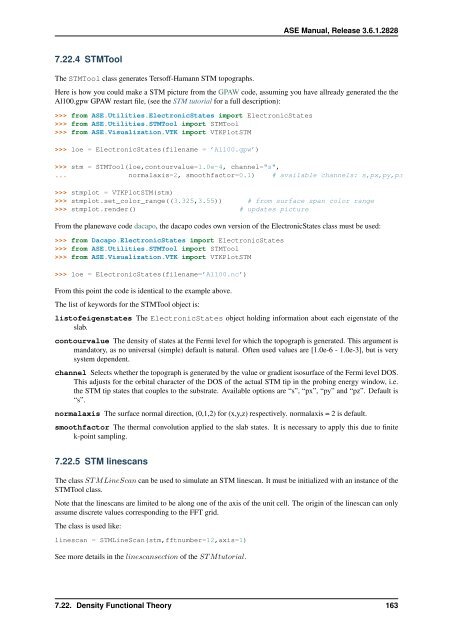
7.22.4 STMTool
The STMTool class generates Tersoff-Hamann STM topographs.
ASE Manual, Release 3.6.1.2828
Here is how you could make a STM picture from the GPAW code, assuming you have allready generated the the
Al100.gpw GPAW restart file, (see the STM tutorial for a full description):
>>> from ASE.Utilities.ElectronicStates import ElectronicStates
>>> from ASE.Utilities.STMTool import STMTool
>>> from ASE.Visualization.VTK import VTKPlotSTM
>>> loe = ElectronicStates(filename = ’Al100.gpw’)
>>> stm = STMTool(loe,contourvalue=1.0e-4, channel="s",
... normalaxis=2, smoothfactor=0.1) # available channels: s,px,py,pz
>>> stmplot = VTKPlotSTM(stm)
>>> stmplot.set_color_range((3.325,3.55)) # from surface span color range
>>> stmplot.render() # updates picture
From the planewave code dacapo, the dacapo codes own version of the ElectronicStates class must be used:
>>> from Dacapo.ElectronicStates import ElectronicStates
>>> from ASE.Utilities.STMTool import STMTool
>>> from ASE.Visualization.VTK import VTKPlotSTM
>>> loe = ElectronicStates(filename=’Al100.nc’)
From this point the code is identical to the example above.
The list of keywords for the STMTool object is:
listofeigenstates The ElectronicStates object holding information about each eigenstate of the
slab.
contourvalue The density of states at the Fermi level for which the topograph is generated. This argument is
mandatory, as no universal (simple) default is natural. Often used values are [1.0e-6 - 1.0e-3], but is very
system dependent.
channel Selects whether the topograph is generated by the value or gradient isosurface of the Fermi level DOS.
This adjusts for the orbital character of the DOS of the actual STM tip in the probing energy window, i.e.
the STM tip states that couples to the substrate. Available options are “s”, “px”, “py” and “pz”. Default is
“s”.
normalaxis The surface normal direction, (0,1,2) for (x,y,z) respectively. normalaxis = 2 is default.
smoothfactor The thermal convolution applied to the slab states. It is necessary to apply this due to finite
k-point sampling.
7.22.5 STM linescans
The class ST MLineScan can be used to simulate an STM linescan. It must be initialized with an instance of the
STMTool class.
Note that the linescans are limited to be along one of the axis of the unit cell. The origin of the linescan can only
assume discrete values corresponding to the FFT grid.
The class is used like:
linescan = STMLineScan(stm,fftnumber=12,axis=1)
See more details in the linescansection of the ST Mtutorial.
7.22. Density Functional Theory 163