To the Graduate Council: I am submitting herewith a thesis written by ...

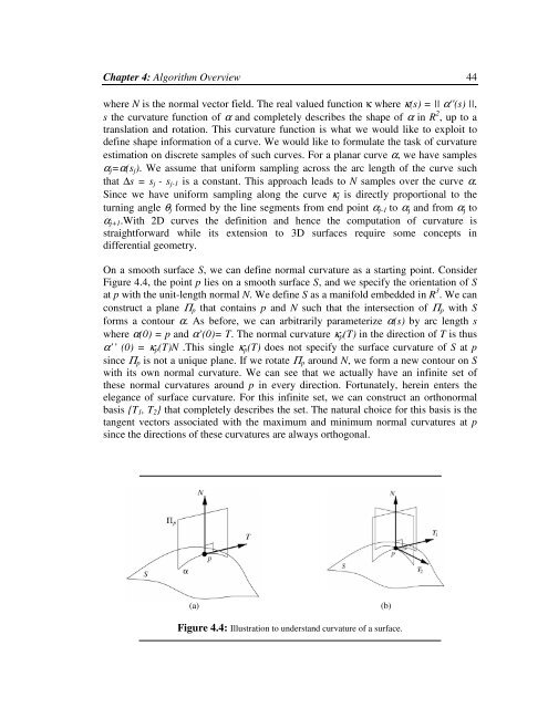
Chapter 4: Algorithm Overview 44where N is the normal vector field. The real valued function κ where κ(s) = || α '(s) ||,s the curvature function of α and completely describes the shape of α in R 2 , up to atranslation and rotation. This curvature function is what we would like to exploit todefine shape information of a curve. We would like to formulate the task of curvatureestimation on discrete samples of such curves. For a planar curve α, we have samplesα j =α(s j ). We assume that uniform sampling across the arc length of the curve suchthat ∆s = s j - s j-1 is a constant. This approach leads to N samples over the curve α.Since we have uniform sampling along the curve κ j is directly proportional to theturning angle θ j formed by the line segments from end point α j-1 to α j and from α j toα j+1 .With 2D curves the definition and hence the computation of curvature isstraightforward while its extension to 3D surfaces require some concepts indifferential geometry.On a smooth surface S, we can define normal curvature as a starting point. ConsiderFigure 4.4, the point p lies on a smooth surface S, and we specify the orientation of Sat p with the unit-length normal N. We define S as a manifold embedded in R 3 . We canconstruct a plane Π p that contains p and N such that the intersection of Π p with Sforms a contour α. As before, we can arbitrarily parameterize α(s) by arc length swhere α(0) = p and α’(0)= T. The normal curvature κ p (T) in the direction of T is thusα’’ (0) = κ p (T)N .This single κ p (T) does not specify the surface curvature of S at psince Π p is not a unique plane. If we rotate Π p around N, we form a new contour on Swith its own normal curvature. We can see that we actually have an infinite set ofthese normal curvatures around p in every direction. Fortunately, herein enters theelegance of surface curvature. For this infinite set, we can construct an orthonormalbasis {T 1 , T 2 } that completely describes the set. The natural choice for this basis is thetangent vectors associated with the maximum and minimum normal curvatures at psince the directions of these curvatures are always orthogonal.(a)(b)Figure 4.4: Illustration to understand curvature of a surface.