To the Graduate Council: I am submitting herewith a thesis written by ...

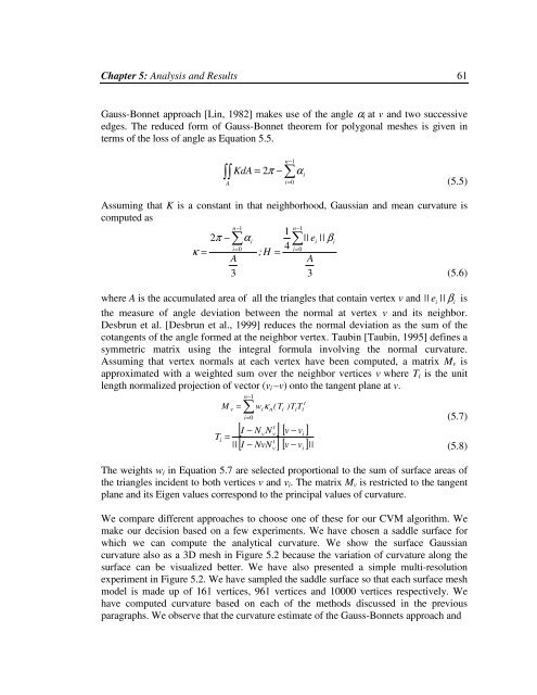
Chapter 5: Analysis and Results 61Gauss-Bonnet approach [Lin, 1982] makes use of the angle α i at v and two successiveedges. The reduced form of Gauss-Bonnet theorem for polygonal meshes is given interms of the loss of angle as Equation 5.5. − KdA = π −i=An 12 α0i(5.5)Assuming that K is a constant in that neighborhood, Gaussian and mean curvature iscomputed asn−1n−112π−αi||ei|| βii= 0 4 i=0κ = ;H =AA33(5.6)where A is the accumulated area of all the triangles that contain vertex v and || e || iβiisthe measure of angle deviation between the normal at vertex v and its neighbor.Desbrun et al. [Desbrun et al., 1999] reduces the normal deviation as the sum of thecotangents of the angle formed at the neighbor vertex. Taubin [Taubin, 1995] defines asymmetric matrix using the integral formula involving the normal curvature.Assuming that vertex normals at each vertex have been computed, a matrix M v isapproximated with a weighted sum over the neighbor vertices v where T i is the unitlength normalized projection of vector (v i –v) onto the tangent plane at v.n 1= − M v wiκn(Ti)TiTii=0Ti=||t[ I − NvNv] [ v − vi]t[ I − NvN ] [ v − v ]||vit(5.7)(5.8)The weights w i in Equation 5.7 are selected proportional to the sum of surface areas ofthe triangles incident to both vertices v and v i . The matrix M v is restricted to the tangentplane and its Eigen values correspond to the principal values of curvature.We compare different approaches to choose one of these for our CVM algorithm. Wemake our decision based on a few experiments. We have chosen a saddle surface forwhich we can compute the analytical curvature. We show the surface Gaussiancurvature also as a 3D mesh in Figure 5.2 because the variation of curvature along thesurface can be visualized better. We have also presented a simple multi-resolutionexperiment in Figure 5.2. We have sampled the saddle surface so that each surface meshmodel is made up of 161 vertices, 961 vertices and 10000 vertices respectively. Wehave computed curvature based on each of the methods discussed in the previousparagraphs. We observe that the curvature estimate of the Gauss-Bonnets approach and