Download Thesis in Pdf Format - Theoretical Nuclear Physics and ...

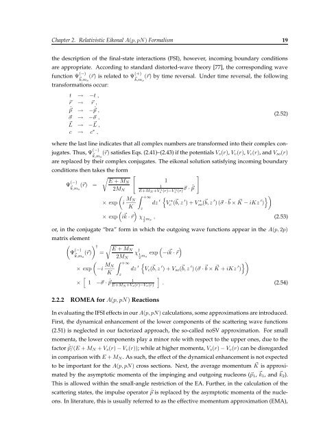
Chapter 2. Relativistic Eikonal A(p, pN) Formalism 19the description of the final-state interactions (FSI), however, incoming boundary conditionsare appropriate. According to standard distorted-wave theory [77], the corresponding wavefunction Ψ (−)⃗(⃗r) is related to Ψ (+)k,ms ⃗(⃗r) by time reversal. Under time reversal, the followingk,mstransformations occur:t → −t ,⃗r → ⃗r ,ˆ⃗p → −ˆ⃗p ,⃗σ → −⃗σ ,⃗L → −L ⃗ ,c → c ∗ ,(2.52)where the last line indicates that all complex numbers are transformed into their complex conjugates.Thus, Ψ (−)⃗ k,ms(⃗r) satisfies Eqs. (2.41)–(2.43) if the potentials V s (r), V v (r), V c (r), and V so (r)are replaced by their complex conjugates. The eikonal solution satisfying incoming boundaryconditions then takes the formΨ (−)⃗ k,ms(⃗r) =√ [E + MN2M N(× exp i M NK(× exp i ⃗ )k · ⃗r11E+M N +Vs ∗ (r)−Vv ∗ (r)∫ +∞z⃗σ · ˆ⃗p]dz ′ { V ∗c ( ⃗ b, z ′ ) + V ∗so( ⃗ b, z ′ ) (⃗σ ·⃗b × ⃗ K − iKz ′ )} )χ 1 , (2.53)ms2or, in the conjugate “bra” form in which the outgoing wave functions appear in the A(p, 2p)matrix element(†√Ψ (−)E + MN(⃗(⃗r))=χ † 1 exp −i k,ms 2M ⃗ )k · ⃗rN 2(ms× exp −i M ∫ +∞ { Ndz ′ V c (K⃗ b, z ′ ) + V so ( ⃗ b, z ′ ) (⃗σ ·⃗b × ⃗ } )K + iKz ′ )z[× 1 −⃗σ · ˆ⃗p]1E+M N +V s(r)−V v(r). (2.54)2.2.2 ROMEA for A(p, pN) ReactionsIn evaluating the IFSI effects in our A(p, pN) calculations, some approximations are introduced.First, the dynamical enhancement of the lower components of the scattering wave functions(2.51) is neglected in our factorized approach, the so-called noSV approximation. For smallmomenta, the lower components play a minor role with respect to the upper ones, due to thefactor ˆ⃗p/(E + M N + V s (r) − V v (r)); while at higher momenta, V s (r) − V v (r) can be disregardedin comparison with E + M N . As such, the effect of the dynamical enhancement is not expectedto be important for the A(p, pN) cross sections. Next, the average momentum ⃗ K is approximatedby the asymptotic momenta of the impinging and outgoing nucleons (⃗p 1 , ⃗ k 1 , and ⃗ k 2 ).This is allowed within the small-angle restriction of the EA. Further, in the calculation of thescattering states, the impulse operator ˆ⃗p is replaced by the asymptotic momenta of the nucleons.In literature, this is usually referred to as the effective momentum approximation (EMA),