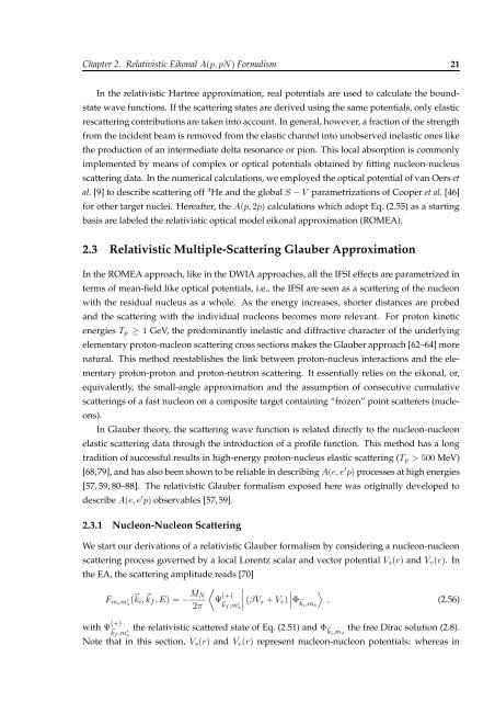
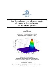
2.2. Relativistic Optical Model Eikonal Approximation 20<strong>in</strong> which the momentum operators that appear <strong>in</strong> sp<strong>in</strong>or-distortion operators are replaced byasymptotic k<strong>in</strong>ematics [78]. As mentioned before, the sp<strong>in</strong>-orbit potential V so is also omitted.As a result, the effects of the <strong>in</strong>teractions of the <strong>in</strong>com<strong>in</strong>g <strong>and</strong> outgo<strong>in</strong>g nucleons withthe residual nucleus are implemented <strong>in</strong> the distorted momentum-space wave function ofEq. (2.35) through the follow<strong>in</strong>g phase factors:Mp R zp1−iŜ p1 (⃗r) = ep 1−∞ dz Vc(⃗ b p1 ,z) ,(2.55a)Mp R−i +∞kŜ k1 (⃗r) = e 1 z dz ′ V c( ⃗ b k1 ,z ′ ) k1 , (2.55b)Ŝ k2 (⃗r) = e −i M Nk2R +∞z k2dz ′′ V c( ⃗ b k2 ,z ′′ ), (2.55c)with the z-axes of the different coord<strong>in</strong>ate systems ly<strong>in</strong>g along the trajectories of the respectiveparticles (z along the direction of the <strong>in</strong>com<strong>in</strong>g proton ⃗p 1 , z ′ along the trajectory of the scatteredproton ⃗ k 1 , <strong>and</strong> z ′′ along the path of the ejected nucleon ⃗ k 2 ); <strong>and</strong> ( ⃗ b p1 , z p1 ), ( ⃗ b k1 , z k1 ), <strong>and</strong> ( ⃗ b k2 , z k2 )are the coord<strong>in</strong>ates of the collision po<strong>in</strong>t ⃗r <strong>in</strong> the respective coord<strong>in</strong>ate systems. The geometryof the A(p, pN) scatter<strong>in</strong>g process is illustrated <strong>in</strong> Fig. 2.3. The <strong>in</strong>tegration limits guarantee thatthe <strong>in</strong>com<strong>in</strong>g proton only undergoes ISI up to the po<strong>in</strong>t where the hard NN collision occurs,<strong>and</strong> the outgo<strong>in</strong>g nucleons are only subject to FSI after this hard collision.k 1z p11p 1b p1b k1b k2 2k 2Figure 2.3 Geometry of the A(p, pN) process. The vectors ⃗ b p1 , ⃗ b k1 , <strong>and</strong> ⃗ b k2 are the impact parameters foreach of the three paths for a collision occurr<strong>in</strong>g at ⃗r. z p1 , z k1 , <strong>and</strong> z k2 are the z coord<strong>in</strong>ates of the collisionpo<strong>in</strong>t <strong>in</strong> the respective coord<strong>in</strong>ate systems. θ 1 <strong>and</strong> θ 2 are the angles of the outgo<strong>in</strong>g nucleons relative tothe <strong>in</strong>com<strong>in</strong>g proton direction.It is worth remark<strong>in</strong>g that the eikonal IFSI operators of Eq. (2.55) are one-body operators,i.e., they do not depend on the coord<strong>in</strong>ates (⃗r 2 , ⃗r 3 , . . . , ⃗r A ) of the residual nucleons. The normalizationof the bound-state wave functions simplifies the IFSI factor (2.36) considerably toŜ IFSI (⃗r) = Ŝk1 (⃗r) Ŝk2 (⃗r) Ŝp1 (⃗r) <strong>in</strong> the ROMEA case.
Chapter 2. Relativistic Eikonal A(p, pN) Formalism 21In the relativistic Hartree approximation, real potentials are used to calculate the boundstatewave functions. If the scatter<strong>in</strong>g states are derived us<strong>in</strong>g the same potentials, only elasticrescatter<strong>in</strong>g contributions are taken <strong>in</strong>to account. In general, however, a fraction of the strengthfrom the <strong>in</strong>cident beam is removed from the elastic channel <strong>in</strong>to unobserved <strong>in</strong>elastic ones likethe production of an <strong>in</strong>termediate delta resonance or pion. This local absorption is commonlyimplemented by means of complex or optical potentials obta<strong>in</strong>ed by fitt<strong>in</strong>g nucleon-nucleusscatter<strong>in</strong>g data. In the numerical calculations, we employed the optical potential of van Oers etal. [9] to describe scatter<strong>in</strong>g off 4 He <strong>and</strong> the global S − V parametrizations of Cooper et al. [46]for other target nuclei. Hereafter, the A(p, 2p) calculations which adopt Eq. (2.55) as a start<strong>in</strong>gbasis are labeled the relativistic optical model eikonal approximation (ROMEA).2.3 Relativistic Multiple-Scatter<strong>in</strong>g Glauber ApproximationIn the ROMEA approach, like <strong>in</strong> the DWIA approaches, all the IFSI effects are parametrized <strong>in</strong>terms of mean-field like optical potentials, i.e., the IFSI are seen as a scatter<strong>in</strong>g of the nucleonwith the residual nucleus as a whole. As the energy <strong>in</strong>creases, shorter distances are probed<strong>and</strong> the scatter<strong>in</strong>g with the <strong>in</strong>dividual nucleons becomes more relevant. For proton k<strong>in</strong>eticenergies T p ≥ 1 GeV, the predom<strong>in</strong>antly <strong>in</strong>elastic <strong>and</strong> diffractive character of the underly<strong>in</strong>gelementary proton-nucleon scatter<strong>in</strong>g cross sections makes the Glauber approach [62–64] morenatural. This method reestablishes the l<strong>in</strong>k between proton-nucleus <strong>in</strong>teractions <strong>and</strong> the elementaryproton-proton <strong>and</strong> proton-neutron scatter<strong>in</strong>g. It essentially relies on the eikonal, or,equivalently, the small-angle approximation <strong>and</strong> the assumption of consecutive cumulativescatter<strong>in</strong>gs of a fast nucleon on a composite target conta<strong>in</strong><strong>in</strong>g “frozen” po<strong>in</strong>t scatterers (nucleons).In Glauber theory, the scatter<strong>in</strong>g wave function is related directly to the nucleon-nucleonelastic scatter<strong>in</strong>g data through the <strong>in</strong>troduction of a profile function. This method has a longtradition of successful results <strong>in</strong> high-energy proton-nucleus elastic scatter<strong>in</strong>g (T p > 500 MeV)[68,79], <strong>and</strong> has also been shown to be reliable <strong>in</strong> describ<strong>in</strong>g A(e, e ′ p) processes at high energies[57, 59, 80–88]. The relativistic Glauber formalism exposed here was orig<strong>in</strong>ally developed todescribe A(e, e ′ p) observables [57, 59].2.3.1 Nucleon-Nucleon Scatter<strong>in</strong>gWe start our derivations of a relativistic Glauber formalism by consider<strong>in</strong>g a nucleon-nucleonscatter<strong>in</strong>g process governed by a local Lorentz scalar <strong>and</strong> vector potential V s (r) <strong>and</strong> V v (r). Inthe EA, the scatter<strong>in</strong>g amplitude reads [70]F msm ′ (⃗ ks i , ⃗ k f , E) = − M 〈NΨ (+)〉2π⃗ kf ,m ′ ∣ (βV ∣s + V v ) ∣Φ ⃗ki ,mss, (2.56)with Ψ (+)⃗ kf ,m ′ sthe relativistic scattered state of Eq. (2.51) <strong>and</strong> Φ ⃗ki ,m sthe free Dirac solution (2.8).Note that <strong>in</strong> this section, V s (r) <strong>and</strong> V v (r) represent nucleon-nucleon potentials; whereas <strong>in</strong>
- Page 1: FACULTEIT WETENSCHAPPENA RELATIVIST
- Page 8 and 9: Contentsiv
- Page 10 and 11: 2mechanism is obtained than in incl
- Page 12 and 13: 4rely on partial-wave expansions of
- Page 15 and 16: Chapter 2Relativistic Eikonal Descr
- Page 18 and 19: 2.1. Observables and Kinematics 10w
- Page 20 and 21: 2.1. Observables and Kinematics 12B
- Page 22 and 23: 2.1. Observables and Kinematics 14M
- Page 24 and 25: 2.1. Observables and Kinematics 16d
- Page 26 and 27: 2.2. Relativistic Optical Model Eik
- Page 30 and 31: 2.3. Relativistic Multiple-Scatteri
- Page 32 and 33: 2.3. Relativistic Multiple-Scatteri
- Page 34 and 35: 2.3. Relativistic Multiple-Scatteri
- Page 36 and 37: 2.4. Approximated RMSGA 2812121010
- Page 38 and 39: 2.5. Second-Order Eikonal Correctio
- Page 40 and 41: 2.5. Second-Order Eikonal Correctio
- Page 42 and 43: 2.5. Second-Order Eikonal Correctio
- Page 44 and 45: 3.1. The IFSI Factor 36sence of ini
- Page 46 and 47: 3.1. The IFSI Factor 38imaginary pa
- Page 48 and 49: 3.2. Radial and Polar-Angle Contrib
- Page 50 and 51: 3.3. A(p, pN) Differential Cross Se
- Page 52 and 53: 3.3. A(p, pN) Differential Cross Se
- Page 54 and 55: 3.3. A(p, pN) Differential Cross Se
- Page 56 and 57: 3.3. A(p, pN) Differential Cross Se
- Page 58 and 59: 3.3. A(p, pN) Differential Cross Se
- Page 60 and 61: 3.3. A(p, pN) Differential Cross Se
- Page 62 and 63: 54Figure 4.1 The beam-momentum depe
- Page 64 and 65: 4.1. High-Momentum-Transfer Wide-An
- Page 66 and 67: 4.1. High-Momentum-Transfer Wide-An
- Page 68 and 69: 4.3. Color Transparency 60of CT. Th
- Page 70 and 71: 4.3. Color Transparency 62with grou
- Page 72 and 73: 4.3. Color Transparency 64with p th
- Page 74 and 75: 4.4. Nuclear Transparency Results 6
- Page 76 and 77: 4.4. Nuclear Transparency Results 6
- Page 78 and 79:
4.4. Nuclear Transparency Results 7
- Page 80 and 81:
4.5. Outlook 72the 7 Li and 12 C da
- Page 82 and 83:
4.5. Outlook 7410.812 C0.6Transpare
- Page 84 and 85:
4.5. Outlook 76
- Page 86 and 87:
5.1. The A(e, e ′ p) Matrix Eleme
- Page 88 and 89:
5.2. Nuclear Transparency 80112 C0.
- Page 90 and 91:
5.3. Induced Normal Polarization 82
- Page 92 and 93:
5.5. Differential Cross Section 84w
- Page 94 and 95:
5.5. Differential Cross Section 860
- Page 96 and 97:
5.5. Differential Cross Section 88d
- Page 98 and 99:
90framework, which is a multiple-sc
- Page 100 and 101:
92be transformed into an amplitude
- Page 102 and 103:
A.2. Pauli Matrices 94A.2 Pauli Mat
- Page 104 and 105:
96pseudo-scalar π mesons, as well
- Page 106 and 107:
980.11ρ chg(e/fm 3 )0.080.060.0440
- Page 108 and 109:
100with∫D r,θ (r, θ) ≡dφ sin
- Page 110 and 111:
Bibliography 102[12] R. A. Arndt, I
- Page 112 and 113:
Bibliography 104[43] E. D. Cooper,
- Page 114 and 115:
Bibliography 106[71] R. J. Glauber,
- Page 116 and 117:
Bibliography 108[104] S. J. Wallace
- Page 118 and 119:
Bibliography 110[132] C. Baglin et
- Page 120 and 121:
Bibliography 112[163] K. Wijesooriy
- Page 122 and 123:
Bibliography 114[195] L. L. Frankfu
- Page 124 and 125:
Bibliography 116[227] J. Botts, J.-
- Page 126 and 127:
Bibliography 118
- Page 128 and 129:
Nederlandstalige samenvatting 120
- Page 130 and 131:
Nederlandstalige samenvatting 122we
- Page 132:
Nederlandstalige samenvatting 1246