Mixture Design Tutorial (Part 1 – The Basics) - Statease.info

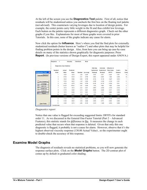
At the left of the screen you see the Diagnostics Tool palette. First of all, notice thatresiduals will be studentized unless you uncheck the first box on the floating tool palette(not advised). This counteracts varying leverages due to location of design points. Forexample, the center points carry little weight in the fit and thus exhibit low leverage.Each button on the palette represents a different diagnostics graph. Check out the othergraphs if you like. Explanations for most of these graphs were covered in priorTutorials. In this case, none of the graphs indicate any cause for alarm.Now click the option for Influence. Here’s where you find the find plots for externallystudentized residuals (better known as “outlier t”) and other plots that may be helpful forfinding problem points in the design. Also, from here you can bring up case-by-casedetails on many of the statistics shown graphically for diagnostic purposes: PressReport. (In previous versions of Design-Expert, this report appeared under ANOVA.)Diagnostics reportNotice that one value is flagged for exceeding suggested limits: DFFITs for standardorder 11. As we discussed in the General One-Factor Tutorial (Part 2 – AdvancedFeatures), this statistic stands for difference in fits. It measures the change in eachpredicted value that occurs when that response is deleted. Given that only this onediagnostic is flagged, it probably is not a cause for alarm. However, observe that it’s thehighest observed viscosity response (130.00 Actual Value) , so the experimenter oughtto double-check the accuracy of this response.Examine Model GraphsThe diagnosis of residuals reveals no statistical problems, so you will now generate theresponse surface plots. Click on the Model Graphs button. The 2D contour plot ofcomes up by default in graduated color shading.14 • Mixture Tutorial – Part 1 Design-Expert 7 User’s Guide