- Page 2:
INTERMEDIATE FINANCIAL MANAGEMENT 9
- Page 6:
Be sure to visit the Intermediate F
- Page 10:
1. The questions indicate to you th
- Page 14:
use a PowerPoint slide show, which
- Page 18:
selected end-of-chapter problems, (
- Page 22:
to the Mini Case slides and Excel f
- Page 26:
publications, along with discussion
- Page 30:
Richard LeCompte Wichita State Univ
- Page 34:
ERRORS IN THE TEXT CONCLUSION At th
- Page 38:
Part 7 Special Topics 830 Chapter 2
- Page 42:
The Efficient Frontier 82, Risk/Ret
- Page 46:
Debt Management Ratios 257 How the
- Page 50:
Box: Corporate Valuation, Cash Flow
- Page 54:
Overview of the Distribution Policy
- Page 58:
Chapter 22 Providing and Obtaining
- Page 62:
Chapter 27 Multinational Financial
- Page 66:
C H A P T E R 1 An Overview of Fina
- Page 70:
advantage in the job market over st
- Page 74:
poor. Of course, there are some con
- Page 78:
Figure 1-1 Sales Revenues Determina
- Page 82:
or a mutual fund manager might base
- Page 86:
owner, the owner/manager will presu
- Page 90:
More and more firms are using a rel
- Page 94:
The second potential conflict occur
- Page 98:
If all of these safeguards were fun
- Page 102:
Self-Test Questions • Section 404
- Page 106:
Inflation Premium (IP) Inflation ha
- Page 110:
The difference between the quoted i
- Page 114:
ankers. Chapter 19 discusses the im
- Page 118:
QUESTIONS • A conflict of interes
- Page 122:
1-2 The real risk-free rate is 3 pe
- Page 126:
IMAGE: © GETTY IMAGES, INC., PHOTO
- Page 130:
CORPORATE VALUATION AND RISK In Cha
- Page 134:
Table 2-1 then, is related to the p
- Page 138:
Figure 2-1 Probability Distribution
- Page 142:
Table 2-3 Calculating Sale.com’s
- Page 146:
When estimated from past data, the
- Page 150:
Self-Test Questions in interest. Al
- Page 154:
Here the ˆr i ’s are the expecte
- Page 158:
Figure 2-5 _ r M(%) 25 15 0 -10 Rat
- Page 162:
Answer: Ford’s and GM’s returns
- Page 166:
THE BENEFITS OF DIVERSIFYING OVERSE
- Page 170:
Figure 2-8 -20 Relative Volatility
- Page 174:
Self-Test Questions on stocks due t
- Page 178:
Table 2-5 Stock Return Data for Gen
- Page 182:
The market risk premium, RP M , sho
- Page 186:
4. The values we worked out for sto
- Page 190:
Figure 2-12 Required Rate of Return
- Page 194:
QUESTIONS • A stock’s beta coef
- Page 198:
2-7 Suppose rRF 9%, rM 14%, and b
- Page 202:
CYBERPROBLEM d. Construct a scatter
- Page 206:
P. Q. Unlimited. Explain how to cal
- Page 210:
B E G I N N I N G - O F - C H A P T
- Page 214:
See IFM9 Ch03 Tool Kit.xls for all
- Page 218:
Using Equation 3-3, the correlation
- Page 222:
Next, we use Equation 3-4 to find
- Page 226:
Self-Test Questions From these exam
- Page 230:
Figure 3-5 Selecting the Optimal Po
- Page 234:
THE CAPITAL MARKET LINE AND THE SEC
- Page 238:
all investors should hold portfolio
- Page 242:
Self-Test Questions Recall that the
- Page 246:
Table 3-4 Figure 3-8 _ _ r = 0.0034
- Page 250:
(r j r RF ) a J b J (r M r RF
- Page 254:
the random error term, e J . Before
- Page 258:
Self-Test Questions 2. Returns may
- Page 262:
Figure 3-10 Required Rate of Return
- Page 266:
The SML states that each stock’s
- Page 270:
Self-Test Questions between low- an
- Page 274:
Self-Test Questions Using the Fama-
- Page 278:
QUESTIONS • The feasible set of p
- Page 282:
a. Construct a scatter diagram show
- Page 286:
SELECTED ADDITIONAL REFERENCES AND
- Page 290:
B E G I N N I N G - O F - C H A P T
- Page 294:
Self-Test Questions bond. Default r
- Page 298:
Provisions to Call or Redeem Bonds
- Page 302:
Self-Test Questions typically requi
- Page 306:
The following general equation, wri
- Page 310:
1 2 3 4 6 Interest Pmt 7 8 9 A Matu
- Page 314:
See IFM9 Ch04 Tool Kit.xls for deta
- Page 318:
You could substitute values for r d
- Page 322:
In 1996 Chateau Teyssier, an Englis
- Page 326:
One’s exposure to interest rate r
- Page 330:
Self-Test Questions DEFAULT RISK Re
- Page 334:
needed $10 million to build a major
- Page 338:
ordinated. Conversely, a bond with
- Page 342:
Table 4-3 types of bonds vary over
- Page 346:
sent to jail. Those events led to t
- Page 350:
and reporting purposes bonds are qu
- Page 354:
QUESTIONS • An adjustment to the
- Page 358:
Bond Yields; Financial Calculator N
- Page 362:
Sam Strother and Shawna Tibbs are v
- Page 366:
IMAGE: © GETTY IMAGES, INC., PHOTO
- Page 370:
CORPORATE VALUATION AND STOCK RISK
- Page 374:
Self-Test Question classifications
- Page 378:
Self-Test Questions RATIONAL EXUBER
- Page 382:
firm’s stock, but the market pric
- Page 386:
Equation 5-2 is the sum of an infin
- Page 390:
profitable investment opportunities
- Page 394:
The popular Motley Fool Web site ht
- Page 398:
ecome a constant growth stock, we c
- Page 402:
STOCK VALUATION BY THE FREE CASH FL
- Page 406:
The investor can calculate Stock i
- Page 410:
the existence of computers and tele
- Page 414:
Self-Test Questions for anyone to c
- Page 418:
Figure 5-5 right indicates how stoc
- Page 422:
Self-Test Questions SUMMARY A NATIO
- Page 426:
QUESTIONS • The marginal investor
- Page 430:
Rates of Return and Equilibrium Sup
- Page 434:
. Now assume that TTC’s period of
- Page 438:
SELECTED ADDITIONAL REFERENCES AND
- Page 442:
B E G I N N I N G - O F - C H A P T
- Page 446:
The Chicago Board Options Exchange
- Page 450:
Figure 6-1 Space Technology Inc.: O
- Page 454:
REPORTING EMPLOYEE STOCK OPTIONS Wh
- Page 458:
Figure 6-2 Current Stock Price $40
- Page 462:
See the Web Extension for this chap
- Page 466:
For a Web-based option calculator,
- Page 470:
d2 d1 0.420.25 0.180 0.20 0.020
- Page 474:
If an employee stock option grant m
- Page 478:
Self-Test Question For example, con
- Page 482:
Self-Test Question SUMMARY would be
- Page 486:
SPREADSHEET PROBLEM Build a Model:
- Page 490:
IMAGE: © GETTY IMAGES, INC., PHOTO
- Page 494:
In Chapter 1, we told you that mana
- Page 498:
THE INCOME STATEMENT See IFM9 Ch07
- Page 502:
See IFM9 Ch07 Tool Kit.xls for deta
- Page 506:
their company’s stock. In additio
- Page 510:
See IFM9 Ch07 Tool Kit.xls for deta
- Page 514:
The first step in modifying the tra
- Page 518:
operating working capital and opera
- Page 522:
chooses. Therefore, we now define a
- Page 526:
Self-Test Questions MVA AND EVA pos
- Page 530:
See IFM9 Ch07 Tool Kit.xls for deta
- Page 534:
THE FEDERAL INCOME TAX SYSTEM See I
- Page 538:
See IFM9 Ch07 Tool Kit.xls for deta
- Page 542:
See the Chapter 7 Web Extension for
- Page 546:
• The statement of retained earni
- Page 550:
PROBLEMS Note: By the time this boo
- Page 554:
Loss Carryback, Carryforward 7-9 Th
- Page 558:
2005 2006 Liabilities and Equity Ac
- Page 562:
IMAGE: © GETTY IMAGES, INC., PHOTO
- Page 566:
CORPORATE VALUATION AND ANALYSIS OF
- Page 570:
Ability to Meet Short-Term Obligati
- Page 574:
year. Annual sales divided by inven
- Page 578:
Self-Test Questions Identify four r
- Page 582:
Self-Test Questions PROFITABILITY R
- Page 586:
firm with the low profit margin mig
- Page 590:
elow the average, this suggests tha
- Page 594:
Table 8-2 MicroDrive Inc.: Summary
- Page 598:
Table 8-4 MicroDrive Inc.: Common S
- Page 602:
e greater than the ROA of 5.7 perce
- Page 606:
Table 8-6 Comparative Ratios for De
- Page 610:
Self-Test Questions tion, which is
- Page 614:
QUESTIONS PROBLEMS • ROE is impor
- Page 618:
Barry Computer Company: Income Stat
- Page 622:
SPREADSHEET PROBLEM Build a Model:
- Page 626:
Income Statements 2005 2006 2007E S
- Page 630:
SELECTED ADDITIONAL REFERENCES AND
- Page 634:
C H A P T E R 9 Financial Planning
- Page 638:
B E G I N N I N G - O F - C H A P T
- Page 642:
sistently outperformed the average
- Page 646:
Figure 9-1 Net Sales ($) 3,000 2,00
- Page 650:
in 2006. The table also shows the h
- Page 654:
See IFM9 Ch09 Tool Kit.xls for deta
- Page 658:
forecasted dividend of 1.08($1.15)
- Page 662:
Forecast Operating Assets As noted
- Page 666:
Based on its required assets and sp
- Page 670:
Self-Test Questions the receivables
- Page 674:
Self-Test Questions Inserting value
- Page 678:
Figure 9-2 a. Constant Ratios Inven
- Page 682:
Self-Test Questions SUMMARY QUESTIO
- Page 686:
Pro Forma Statements and Ratios Add
- Page 690:
9-9 The Booth Company’s sales are
- Page 694:
B. 2006 INCOME S TATEMENT (MILLIONS
- Page 698:
IMAGE: © GETTY IMAGES, INC., PHOTO
- Page 702:
CORPORATE VALUATION AND THE COST OF
- Page 706:
Self-Test Questions and it is also
- Page 710:
Self-Test Questions THE CAPM APPROA
- Page 714:
Go to http://investor.reuters .com,
- Page 718:
To find an estimate of beta, go to
- Page 722:
Self-Test Questions estimate the ma
- Page 726:
For example, see http://www.zacks.c
- Page 730:
Self-Test Question dents used the C
- Page 734:
Self-Test Questions GLOBAL VARIATIO
- Page 738:
ADJUSTING THE COST OF CAPITAL FOR R
- Page 742:
Self-Test Questions company’s cos
- Page 746:
ADJUSTING THE COST OF CAPITAL FOR F
- Page 750:
Self-Test Questions Table 10-1 Aver
- Page 754:
To find the current S&P 500 market
- Page 758:
QUESTIONS banker helps the company
- Page 762:
10-9 The Bouchard Company’s curre
- Page 766:
Flotation Costs and the Cost of Equ
- Page 770:
(2) Should the component costs be f
- Page 774:
IMAGE: © GETTY IMAGES, INC., PHOTO
- Page 778:
CORPORATE VALUATION: PUTTING THE PI
- Page 782:
plants, patents, and other real ass
- Page 786:
Table 11-2 MagnaVision Inc.: Balanc
- Page 790:
A variant of the constant growth di
- Page 794:
Table 11-4 Finding the Value of Mag
- Page 798:
Table 11-5 Financial Results for Be
- Page 802:
Table 11-7 Initial Projections for
- Page 806:
See IFM9 Ch11 Tool Kit.xls for all
- Page 810:
Table 11-9 Bell Electronics’ Fore
- Page 814:
VALUE-BASED MANAGEMENT IN PRACTICE
- Page 818:
een in power for a long time, and i
- Page 822:
Executive bonuses are based on a nu
- Page 826:
Executive compensation packages dif
- Page 830:
G&A’s Balance Sheet after the ESO
- Page 834:
Self-Test Questions SUMMARY What ar
- Page 838:
PROBLEMS 11-4 What are some actions
- Page 842:
11-9 The balance sheets of Roop Ind
- Page 846:
Balance Sheets for December 31 (Mil
- Page 850:
k. What is the expected ROIC of eac
- Page 854:
C H A P T E R 1 2 Capital Budgeting
- Page 858:
B E G I N N I N G - O F - C H A P T
- Page 862:
PROJECT CLASSIFICATIONS Self-Test Q
- Page 866:
Figure 12-2 Project S: Net cash flo
- Page 870:
The equation for the NPV is as foll
- Page 874:
project’s future EVAs. Therefore,
- Page 878:
Self-Test Questions What four capit
- Page 882:
capital is greater than 11.8 percen
- Page 886:
Self-Test Questions When solved, we
- Page 890:
Self-Test Questions PROFITABILITY I
- Page 894:
an expected payoff of $115,500 afte
- Page 898:
Self-Test Question THE POST-AUDIT A
- Page 902:
Figure 12-6 Project C: 0 Comparing
- Page 906:
Economic Life versus Physical Life
- Page 910:
Self-Test Questions 1. Reluctance t
- Page 914:
QUESTIONS • Small firms tend to u
- Page 918:
Capital Budgeting Methods 12-5 Proj
- Page 922:
Present Value of Costs Payback, NPV
- Page 926:
SPREADSHEET PROBLEM Build a Model:
- Page 930:
(2) Look at your NPV profile graph
- Page 934:
IMAGE: © GETTY IMAGES, INC., PHOTO
- Page 938: CORPORATE VALUATION, CASH FLOWS, AN
- Page 942: eceivables. The difference between
- Page 946: See IFM9 Ch13 Tool Kit.xls for all
- Page 950: stockholder reporting, one normally
- Page 954: Table 13-3 Recovery Allowance Perce
- Page 958: 3. Terminal year cash flow. At the
- Page 962: Table 13-4 75 76 77 78 79 80 81 82
- Page 966: Table 13-4 119 120 121 122 123 124
- Page 970: Suppose the expected rate of inflat
- Page 974: somewhat higher or lower than 20,00
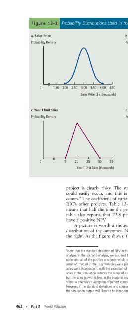
- Page 978: Table 13-5 or low sales prices and
- Page 982: CAPITAL BUDGETING PRACTICES IN THE
- Page 986: ound of $1.40, a most likely value
- Page 992: PROJECT RISK CONCLUSIONS Self-Test
- Page 996: Figure 13-4 466 • Part 3 Project
- Page 1000: 468 • Part 3 Project Valuation Co
- Page 1004: Self-Test Question SUMMARY 470 •
- Page 1008: PROBLEMS 472 • Part 3 Project Val
- Page 1012: 13-8 The Bartram-Pulley Company (BP
- Page 1016: SPREADSHEET PROBLEM Build a Model:
- Page 1020: (3) Use the worst-, most likely, an
- Page 1024: B E G I N N I N G - O F - C H A P T
- Page 1028: THE INVESTMENT TIMING OPTION: AN IL
- Page 1032: 484 • Part 3 Project Valuation Ap
- Page 1036: 486 • Part 3 Project Valuation In
- Page 1040:
Figure 14-3 Notes: a The WACC is 14
- Page 1044:
Figure 14-4 PART 1. FIND THE VALUE
- Page 1048:
Figure 14-5 Self-Test Questions 492
- Page 1052:
494 • Part 3 Project Valuation of
- Page 1056:
Table 14-1 Cost of Capital Used to
- Page 1060:
GROWTH OPTIONS AT DOT-COM COMPANIES
- Page 1064:
CONCLUDING THOUGHTS ON REAL OPTIONS
- Page 1068:
PROBLEMS Investment Timing Option:
- Page 1072:
Growth Option: Option Analysis 504
- Page 1076:
partfour Strategic Financing Decisi
- Page 1080:
C H A P T E R 15 Capital Structure
- Page 1084:
A firm’s financing choices obviou
- Page 1088:
Self-Test Question 512 • Part 4 S
- Page 1092:
See IFM9 Ch15 Tool Kit.xls for deta
- Page 1096:
Figure 15-1 Revenues and Costs (Tho
- Page 1100:
Table 15-1 Section I. Zero Debt Deb
- Page 1104:
520 • Part 4 Strategic Financing
- Page 1108:
522 • Part 4 Strategic Financing
- Page 1112:
Figure 15-2 524 • Part 4 Strategi
- Page 1116:
526 • Part 4 Strategic Financing
- Page 1120:
528 • Part 4 Strategic Financing
- Page 1124:
Self-Test Questions 530 • Part 4
- Page 1128:
532 • Part 4 Strategic Financing
- Page 1132:
Figure 15-3 534 • Part 4 Strategi
- Page 1136:
Table 15-4 536 • Part 4 Strategic
- Page 1140:
538 • Part 4 Strategic Financing
- Page 1144:
Self-Test Questions SUMMARY 540 •
- Page 1148:
PROBLEMS 542 • Part 4 Strategic F
- Page 1152:
WACC and Optimal Capital Structure
- Page 1156:
h. With the above points in mind, n
- Page 1160:
C H A P T E R 16 Capital Structure
- Page 1164:
This chapter extends the discussion
- Page 1168:
552 • Part 4 Strategic Financing
- Page 1172:
554 • Part 4 Strategic Financing
- Page 1176:
556 • Part 4 Strategic Financing
- Page 1180:
Figure 16-1 a. Without Taxes Cost o
- Page 1184:
INTRODUCING PERSONAL TAXES: THE MIL
- Page 1188:
562 • Part 4 Strategic Financing
- Page 1192:
564 • Part 4 Strategic Financing
- Page 1196:
566 • Part 4 Strategic Financing
- Page 1200:
Self-Test Questions 568 • Part 4
- Page 1204:
For Kunkel Inc., 570 • Part 4 Str
- Page 1208:
Table 16-2 572 • Part 4 Strategic
- Page 1212:
Figure 16-2 574 • Part 4 Strategi
- Page 1216:
QUESTIONS 576 • Part 4 Strategic
- Page 1220:
16-3 Refer to Problem 16-2. Assume
- Page 1224:
David Lyons, CEO of Lyons Solar Tec
- Page 1228:
C H A P T E R 17 Distributions to S
- Page 1232:
CORPORATE VALUATION AND DISTRIBUTIO
- Page 1236:
586 • Part 4 Strategic Financing
- Page 1240:
DIVIDEND YIELDS AROUND THE WORLD Di
- Page 1244:
INFORMATION CONTENT, OR SIGNALING,
- Page 1248:
Table 17-1 592 • Part 4 Strategic
- Page 1252:
Self-Test Question Table 17-2 594
- Page 1256:
Self-Test Questions 596 • Part 4
- Page 1260:
598 • Part 4 Strategic Financing
- Page 1264:
See IFM9 Ch17 Tool Kit.xls for all
- Page 1268:
Self-Test Questions 602 • Part 4
- Page 1272:
604 • Part 4 Strategic Financing
- Page 1276:
606 • Part 4 Strategic Financing
- Page 1280:
Self-Test Questions SUMMARY 608 •
- Page 1284:
PROBLEMS Residual Distribution Mode
- Page 1288:
Alternative Dividend Policies 612
- Page 1292:
(3) What are the advantages and dis
- Page 1296:
partfive Tactical Financing Decisio
- Page 1300:
C H A P T E R 18 Initial Public Off
- Page 1304:
CORPORATE VALUATION, IPOs, AND FINA
- Page 1308:
622 • Part 5 Tactical Financing D
- Page 1312:
624 • Part 5 Tactical Financing D
- Page 1316:
626 • Part 5 Tactical Financing D
- Page 1320:
628 • Part 5 Tactical Financing D
- Page 1324:
630 • Part 5 Tactical Financing D
- Page 1328:
Self-Test Questions 632 • Part 5
- Page 1332:
634 • Part 5 Tactical Financing D
- Page 1336:
Self-Test Questions 636 • Part 5
- Page 1340:
Self-Test Questions 638 • Part 5
- Page 1344:
Self-Test Questions 640 • Part 5
- Page 1348:
Table 18-3 13 14 15 16 17 18 19 20
- Page 1352:
644 • Part 5 Tactical Financing D
- Page 1356:
646 • Part 5 Tactical Financing D
- Page 1360:
648 • Part 5 Tactical Financing D
- Page 1364:
Self-Test Questions 650 • Part 5
- Page 1368:
QUESTIONS PROBLEMS 652 • Part 5 T
- Page 1372:
654 • Part 5 Tactical Financing D
- Page 1376:
Randy’s, a family-owned restauran
- Page 1380:
C H A P T E R 19 Lease Financing Th
- Page 1384:
Leasing is another form of financin
- Page 1388:
662 • Part 5 Tactical Financing D
- Page 1392:
Self-Test Questions 664 • Part 5
- Page 1396:
Self-Test Questions 666 • Part 5
- Page 1400:
668 • Part 5 Tactical Financing D
- Page 1404:
Table 19-2 670 • Part 5 Tactical
- Page 1408:
See IFM9 Ch19 Tool Kit.xls. 672 •
- Page 1412:
674 • Part 5 Tactical Financing D
- Page 1416:
676 • Part 5 Tactical Financing D
- Page 1420:
Self-Test Question 678 • Part 5 T
- Page 1424:
PROBLEMS 680 • Part 5 Tactical Fi
- Page 1428:
Build a Model: Lessee’s Analysis
- Page 1432:
ut that $200,000 is the expected va
- Page 1436:
C H A P T E R 20 Hybrid Financing:
- Page 1440:
Preferred stock, warrants, and conv
- Page 1444:
Suppose your company needs cash to
- Page 1448:
692 • Part 5 Tactical Financing D
- Page 1452:
694 • Part 5 Tactical Financing D
- Page 1456:
See IFM9 Ch20 Tool Kit.xls. 696 •
- Page 1460:
698 • Part 5 Tactical Financing D
- Page 1464:
700 • Part 5 Tactical Financing D
- Page 1468:
Figure 20-1 702 • Part 5 Tactical
- Page 1472:
704 • Part 5 Tactical Financing D
- Page 1476:
706 • Part 5 Tactical Financing D
- Page 1480:
Self-Test Questions 708 • Part 5
- Page 1484:
PROBLEMS 710 • Part 5 Tactical Fi
- Page 1488:
712 • Part 5 Tactical Financing D
- Page 1492:
Because he expects earnings to cont
- Page 1496:
partsix Working Capital Management
- Page 1500:
C H A P T E R 21 Working Capital Ma
- Page 1504:
Superior working capital management
- Page 1508:
722 • Part 6 Working Capital Mana
- Page 1512:
Self-Test Questions Table 21-1 724
- Page 1516:
THE BEST AT MANAGING WORKING CAPITA
- Page 1520:
See IFM9 Ch21 Tool Kit.xls for all
- Page 1524:
THE GREAT DEBATE: HOW MUCH CASH IS
- Page 1528:
732 • Part 6 Working Capital Mana
- Page 1532:
Self-Test Question 734 • Part 6 W
- Page 1536:
736 • Part 6 Working Capital Mana
- Page 1540:
Self-Test Questions Table 21-3 738
- Page 1544:
740 • Part 6 Working Capital Mana
- Page 1548:
Self-Test Questions 742 • Part 6
- Page 1552:
Self-Test Questions 744 • Part 6
- Page 1556:
SHORT-TERM FINANCING Self-Test Ques
- Page 1560:
Self-Test Question 748 • Part 6 W
- Page 1564:
Self-Test Questions SUMMARY 750 •
- Page 1568:
QUESTIONS 752 • Part 6 Working Ca
- Page 1572:
21-6 McDowell Industries sells on t
- Page 1576:
756 • Part 6 Working Capital Mana
- Page 1580:
Dan Barnes, financial manager of Sk
- Page 1584:
f. In his preliminary cash budget,
- Page 1588:
C H A P T E R 22 Providing and Obta
- Page 1592:
CORPORATE VALUATION AND CREDIT POLI
- Page 1596:
SETTING THE COLLECTION POLICY Self-
- Page 1600:
Table 22-1 768 • Part 6 Working C
- Page 1604:
Table 22-2 770 • Part 6 Working C
- Page 1608:
Self-Test Questions 772 • Part 6
- Page 1612:
Self-Test Questions 774 • Part 6
- Page 1616:
776 • Part 6 Working Capital Mana
- Page 1620:
778 • Part 6 Working Capital Mana
- Page 1624:
780 • Part 6 Working Capital Mana
- Page 1628:
782 • Part 6 Working Capital Mana
- Page 1632:
784 • Part 6 Working Capital Mana
- Page 1636:
786 • Part 6 Working Capital Mana
- Page 1640:
788 • Part 6 Working Capital Mana
- Page 1644:
QUESTIONS 790 • Part 6 Working Ca
- Page 1648:
22-4 On March 1, Minnerly Motors ob
- Page 1652:
794 • Part 6 Working Capital Mana
- Page 1656:
e. What is the firm’s forecasted
- Page 1660:
SELECTED ADDITIONAL REFERENCES AND
- Page 1664:
B E G I N N I N G - O F - C H A P T
- Page 1668:
Self-Test Question 802 • Part 6 W
- Page 1672:
804 • Part 6 Working Capital Mana
- Page 1676:
806 • Part 6 Working Capital Mana
- Page 1680:
INVENTORY CONTROL SYSTEMS 808 • P
- Page 1684:
ACCOUNTING FOR INVENTORY 810 • Pa
- Page 1688:
THE ECONOMIC ORDERING QUANTITY (EOQ
- Page 1692:
814 • Part 6 Working Capital Mana
- Page 1696:
816 • Part 6 Working Capital Mana
- Page 1700:
Self-Test Questions 818 • Part 6
- Page 1704:
Table 23-1 820 • Part 6 Working C
- Page 1708:
822 • Part 6 Working Capital Mana
- Page 1712:
Self-Test Questions Why are safety
- Page 1716:
PROBLEMS Economic Ordering Quantity
- Page 1720:
Andria Mullins, financial manager o
- Page 1724:
partseven Special Topics
- Page 1728:
C H A P T E R 24 Derivatives and Ri
- Page 1732:
Risk management can reduce firm ris
- Page 1736:
836 • Part 7 Special Topics finan
- Page 1740:
Self-Test Questions 838 • Part 7
- Page 1744:
840 • Part 7 Special Topics fluct
- Page 1748:
842 • Part 7 Special Topics Forwa
- Page 1752:
844 • Part 7 Special Topics Figur
- Page 1756:
846 • Part 7 Special Topics bonds
- Page 1760:
Self-Test Question RISK MANAGEMENT
- Page 1764:
MICROSOFT’S GOAL: MANAGE EVERY RI
- Page 1768:
Table 24-2 852 • Part 7 Special T
- Page 1772:
854 • Part 7 Special Topics Futur
- Page 1776:
856 • Part 7 Special Topics and i
- Page 1780:
858 • Part 7 Special Topics the c
- Page 1784:
QUESTIONS PROBLEMS 860 • Part 7 S
- Page 1788:
Assume that you have just been hire
- Page 1792:
C H A P T E R 25 Bankruptcy, Reorga
- Page 1796:
CORPORATE VALUATION AND BANKRUPTCY
- Page 1800:
Table 25-2 ISSUES FACING A FIRM IN
- Page 1804:
870 • Part 7 Special Topics as a
- Page 1808:
Self-Test Questions 872 • Part 7
- Page 1812:
874 • Part 7 Special Topics subsi
- Page 1816:
876 • Part 7 Special Topics The p
- Page 1820:
Table 25-4 878 • Part 7 Special T
- Page 1824:
880 • Part 7 Special Topics sold
- Page 1828:
882 • Part 7 Special Topics What
- Page 1832:
Table 25-6 884 • Part 7 Special T
- Page 1836:
Self-Test Question 886 • Part 7 S
- Page 1840:
QUESTIONS 888 • Part 7 Special To
- Page 1844:
890 • Part 7 Special Topics singl
- Page 1848:
of directors. In turn, Ron asked yo
- Page 1852:
C H A P T E R 26 Mergers, LBOs, Div
- Page 1856:
CORPORATE VALUATION AND MERGERS The
- Page 1860:
898 • Part 7 Special Topics merge
- Page 1864:
TYPES OF MERGERS Self-Test Question
- Page 1868:
Self-Test Questions 902 • Part 7
- Page 1872:
Self-Test Questions 904 • Part 7
- Page 1876:
906 • Part 7 Special Topics The v
- Page 1880:
Self-Test Questions 908 • Part 7
- Page 1884:
Table 26-2 910 • Part 7 Special T
- Page 1888:
Table 26-3 912 • Part 7 Special T
- Page 1892:
See IFM9 Ch26 Tool Kit.xls for deta
- Page 1896:
Self-Test Questions SETTING THE BID
- Page 1900:
918 • Part 7 Special Topics The E
- Page 1904:
920 • Part 7 Special Topics In a
- Page 1908:
Figure 26-2 Mostly cash Note: These
- Page 1912:
See IFM9 Ch26 Tool Kit.xls for deta
- Page 1916:
Self-Test Questions 926 • Part 7
- Page 1920:
928 • Part 7 Special Topics stake
- Page 1924:
Self-Test Questions CORPORATE ALLIA
- Page 1928:
932 • Part 7 Special Topics priva
- Page 1932:
Self-Test Questions HOLDING COMPANI
- Page 1936:
Self-Test Questions SUMMARY 936 •
- Page 1940:
PROBLEMS 938 • Part 7 Special Top
- Page 1944:
Build a Model: Merger Analysis 940
- Page 1948:
offer for Lyons Lighting? If so, ho
- Page 1952:
C H A P T E R 27 Multinational Fina
- Page 1956:
The special issues facing a multina
- Page 1960:
MULTINATIONAL VERSUS DOMESTIC FINAN
- Page 1964:
The Bloomberg World Currency Values
- Page 1968:
Table 27-2 952 • Part 7 Special T
- Page 1972:
954 • Part 7 Special Topics For e
- Page 1976:
956 • Part 7 Special Topics gover
- Page 1980:
Table 27-3 Notes: aThese are repres
- Page 1984:
HUNGRY FOR A BIG MAC? GO TO THE PHI
- Page 1988:
Self-Test Question 962 • Part 7 S
- Page 1992:
Self-Test Questions 964 • Part 7
- Page 1996:
Self-Test Questions 966 • Part 7
- Page 2000:
Table 27-4 968 • Part 7 Special T
- Page 2004:
STOCK MARKET INDICES AROUND THE WOR
- Page 2008:
Table 27-6 972 • Part 7 Special T
- Page 2012:
974 • Part 7 Special Topics equip
- Page 2016:
Self-Test Questions SUMMARY 976 •
- Page 2020:
QUESTIONS 978 • Part 7 Special To
- Page 2024:
980 • Part 7 Special Topics On th
- Page 2028:
and 4 percent in Spain. Does intere
- Page 2032:
appendix b Answers to End-of-Chapte
- Page 2036:
8-9 a. Current ratio 1.98; DSO 76
- Page 2040:
15-4 30% debt: WACC 11.14%; V $10
- Page 2044:
23-1 a. 3,000 bags. b. 4,000 bags.
- Page 2048:
n p B a (rpi rˆ p) i1 2Pi . bi
- Page 2052:
994 • Appendix C Selected Equatio
- Page 2056:
996 • Appendix C Selected Equatio
- Page 2060:
Chapter 13 n NPV a t0 n NPV B a i
- Page 2064:
V Tax shield r dTD r TS g . VL V
- Page 2068:
TCC (C)(P)(A). TOC (F)(N) F(S/2A
- Page 2072:
annuity due An annuity with payment
- Page 2076:
coefficient of variation (CV) Equal
- Page 2080:
the percentage of funds provided by
- Page 2084:
eturn will equal the expected rate
- Page 2088:
improper accumulation The retention
- Page 2092:
stock) and the book value of the fi
- Page 2096:
operating leverage The extent to wh
- Page 2100:
lessors. The most important aspect
- Page 2104:
presentations in 10 to 20 cities, w
- Page 2108:
tax preference theory Proposes that
- Page 2112:
name index Abreo, Leslie, 645n Acke
- Page 2116:
subject index AAII. See American As
- Page 2120:
Capital budgeting, 396, 398 in Asia
- Page 2124:
DaimlerChrysler AG, 867 Dalkon Shie
- Page 2128:
Financial reporting, 214-216. See a
- Page 2132:
Kashima Oil, 858-859 Keiretsus, 380
- Page 2136:
Opportunity costs, 233, 323, 440 as
- Page 2140:
Risk, (continued) project, 435, 464
- Page 2144:
TVA, interest expenses of, 645 Two-