- Page 1 and 2: EXAMPLE 17: Full.Coupled Diffusion
- Page 3 and 4: EXAMPLE 17: Full.Coupled Diffusion
- Page 5 and 6: EXAMPLE 16: Two.Dim Diffusion With
- Page 7 and 8: EXAMPLE 16: Two.Dim Diffusion With
- Page 9 and 10: EXAMPLE 15: Annealing An Implant Fr
- Page 11 and 12: EXAMPLE 14: Grown-in and Annealed B
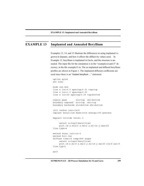
- Page 13: EXAMPLE 13: Implanted and Annealed
- Page 17 and 18: EXAMPLE 12: Dopant Activation Model
- Page 19 and 20: EXAMPLE 11: GaAs Simulation - 2D 29
- Page 21 and 22: EXAMPLE 11: GaAs Simulation - 2D im
- Page 23 and 24: EXAMPLE 10: GaAs MESFET Gate Simula
- Page 25 and 26: EXAMPLE 10: GaAs MESFET Gate Simula
- Page 27 and 28: EXAMPLE 9: Stress Dependent Oxidati
- Page 29 and 30: EXAMPLE 9: Stress Dependent Oxidati
- Page 31 and 32: EXAMPLE 9: Stress Dependent Oxidati
- Page 33 and 34: EXAMPLE 8: Shear Stress FIGURE 1 Cr
- Page 35 and 36: EXAMPLE 8: Shear Stress line y loc=
- Page 37 and 38: EXAMPLE 7: Fully Recessed Oxide Gro
- Page 39 and 40: EXAMPLE 7: Fully Recessed Oxide Gro
- Page 41 and 42: EXAMPLE 7: Fully Recessed Oxide Gro
- Page 43 and 44: EXAMPLE 6: One Dimensional Oxide Gr
- Page 45 and 46: EXAMPLE 6: One Dimensional Oxide Gr
- Page 47 and 48: EXAMPLE 5: LDD Cross Section 266 SU
- Page 49 and 50: EXAMPLE 5: LDD Cross Section To pre
- Page 51 and 52: EXAMPLE 5: LDD Cross Section This i
- Page 53 and 54: EXAMPLE 5: LDD Cross Section The ne
- Page 55 and 56: EXAMPLE 5: LDD Cross Section #depos
- Page 57 and 58: EXAMPLE 4: Boron OED - 2D 256 SUPRE
- Page 59 and 60: EXAMPLE 4: Boron OED - 2D FIGURE 3
- Page 61 and 62: EXAMPLE 4: Boron OED - 2D equal to
- Page 63 and 64: EXAMPLE 4: Boron OED - 2D deposit o
- Page 65 and 66:
EXAMPLE 3: OED Time 248 SUPREM-IV.G
- Page 67 and 68:
EXAMPLE 3: OED Time %define den ${t
- Page 69 and 70:
EXAMPLE 3: OED Time %define tfci 0.
- Page 71 and 72:
EXAMPLE 2: Boron OED - 1D 242 SUPRE
- Page 73 and 74:
EXAMPLE 2: Boron OED - 1D than the
- Page 75 and 76:
EXAMPLE 2: Boron OED - 1D select z=
- Page 77 and 78:
EXAMPLE 1: Boron Anneal - 1D 236 SU
- Page 79 and 80:
EXAMPLE 1: Boron Anneal - 1D Solvin
- Page 81 and 82:
EXAMPLE 1: Boron Anneal - 1D The ne
- Page 83 and 84:
EXAMPLE 1: Boron Anneal - 1D #save
- Page 85 and 86:
Examples 228 SUPREM-IV.GS - 2D Proc
- Page 87 and 88:
ZINC 226 SUPREM-IV.GS - 2D Process
- Page 89 and 90:
ZINC ss.temp, ss.conc These paramet
- Page 91 and 92:
ZINC librium value, D V and D I are
- Page 93 and 94:
VACANCY promising with these models
- Page 95 and 96:
VACANCY vmole, theta.0, theta.E, Gp
- Page 97 and 98:
VACANCY Kr.0, Kr.E These floating p
- Page 99 and 100:
VACANCY DESCRIPTION This statement
- Page 101 and 102:
TRAP BUGS There are no known bugs i
- Page 103 and 104:
TRAP COMMAND TRAP Set coefficients
- Page 105 and 106:
TIN ss.temp, ss.conc These paramete
- Page 107 and 108:
TIN tration and the intrinsic conce
- Page 109 and 110:
iSILICON SEE ALSO The antimony, ars
- Page 111 and 112:
iSILICON ss.clear This parameter cl
- Page 113 and 114:
iSILICON diffusivities with vacanci
- Page 115 and 116:
SELENIUM selenium gaas /nitride Seg
- Page 117 and 118:
SELENIUM faults to 0.0 eV [1,2,3].
- Page 119 and 120:
SELENIUM COMMAND SELENIUM Set the c
- Page 121 and 122:
PHOSPHORUS Trn.0, Trn.E These param
- Page 123 and 124:
PHOSPHORUS Dix.0, Dix.E These float
- Page 125 and 126:
PHOSPHORUS COMMAND PHOSPHORUS Set t
- Page 127 and 128:
OXIDE erf.lbb The erf.lbb parameter
- Page 129 and 130:
OXIDE stress.dep, Vc, Vr, Vd, Vt, D
- Page 131 and 132:
OXIDE dry | wet The type of oxidati
- Page 133 and 134:
OXIDE COMMAND OXIDE Specify oxidati
- Page 135 and 136:
MATERIAL lcte This is an expression
- Page 137 and 138:
MATERIAL COMMAND MATERIAL Set the c
- Page 139 and 140:
MAGNESIUM EXAMPLES magnesium gaas i
- Page 141 and 142:
MAGNESIUM arsenide, and Dix.E defau
- Page 143 and 144:
MAGNESIUM COMMAND MAGNESIUM Set the
- Page 145 and 146:
INTERSTITIAL unknown dependencies o
- Page 147 and 148:
INTERSTITIAL terial. Once again, th
- Page 149 and 150:
* CI = CStar INTERSTITIAL neu.0, ne
- Page 151 and 152:
INTERSTITIAL where C T is the total
- Page 153 and 154:
INTERSTITIAL COMMAND INTERSTITIAL S
- Page 155 and 156:
GERMANIUM ss.temp, ss.conc These pa
- Page 157 and 158:
GERMANIUM tron concentration and th
- Page 159 and 160:
GENERIC donor, acceptor These param
- Page 161 and 162:
GENERIC Dimmm.0, Dimmm.E These floa
- Page 163 and 164:
GENERIC C T t = 150 SUPREM-IV.GS -
- Page 165 and 166:
CARBON EXAMPLES carbon gaas implant
- Page 167 and 168:
CARBON Dix.E is the activation ener
- Page 169 and 170:
CARBON COMMAND CARBON Set the coeff
- Page 171 and 172:
BORON donor, acceptor These paramet
- Page 173 and 174:
BORON and Dix.E defaults to 3.46 eV
- Page 175 and 176:
BORON COMMAND BORON Set the coeffic
- Page 177 and 178:
BERYLLIUM EXAMPLES beryllium gaas i
- Page 179 and 180:
BERYLLIUM Dix.0, Dix.E These floati
- Page 181 and 182:
BERYLLIUM COMMAND BERYLLIUM Set the
- Page 183 and 184:
ARSENIC EXAMPLES arsenic silicon Di
- Page 185 and 186:
ARSENIC and Dix.E defaults to 3.65
- Page 187 and 188:
ARSENIC COMMAND ARSENIC Set the coe
- Page 189 and 190:
ANTIMONY /silicon, /oxide, /oxynit,
- Page 191 and 192:
ANTIMONY and interstitials, and n a
- Page 193 and 194:
Models BUGS These commands implemen
- Page 195 and 196:
STRUCTURE structure imagetool=foo x
- Page 197 and 198:
STRUCTURE pixely This integer param
- Page 199 and 200:
STRUCTURE SCES (Sept. 87 version).
- Page 201 and 202:
STRESS BUGS The correct boundary co
- Page 203 and 204:
SELECT select z=(phos - 5.0e14) Cho
- Page 205 and 206:
SELECT ci.star equilibrium intersti
- Page 207 and 208:
REGION EXAMPLES region silicon xlo=
- Page 209 and 210:
PROFILE antimony, arsenic, boron, p
- Page 211 and 212:
PRINTF printf ( 15.0 * exp ( -2.0 /
- Page 213 and 214:
PRINT.1D EXAMPLES print.1d x.val=1.
- Page 215 and 216:
PRINT.1D COMMAND PRINT.1D Print val
- Page 217 and 218:
PLOT.2D line.grid The line.grid par
- Page 219 and 220:
PLOT.2D COMMAND PLOT.2D Plot a two
- Page 221 and 222:
PLOT.1D clear The clear parameter s
- Page 223 and 224:
PLOT.1D COMMAND PLOT.1D Plot a one
- Page 225 and 226:
OPTION COMMAND OPTION option - Set
- Page 227 and 228:
METHOD REFERENCES 1. M.E. Law and R
- Page 229 and 230:
METHOD fies the percentage of the t
- Page 231 and 232:
METHOD blk.itlim The maximum number
- Page 233 and 234:
METHOD plexity desired for the diff
- Page 235 and 236:
LINE BUGS It's hard to guess how ma
- Page 237 and 238:
LINE COMMAND LINE Specify a mesh li
- Page 239 and 240:
LABEL COMMAND LABEL Put labels on a
- Page 241 and 242:
INITIALIZE antimony, arsenic, beryl
- Page 243 and 244:
IMPLANT Occasionally problems are e
- Page 245 and 246:
IMPLANT antimony, arsenic, boron, b
- Page 247 and 248:
ETCH EXAMPLES etch nitride left p1.
- Page 249 and 250:
ETCH COMMAND ETCH Etch a layer. SYN
- Page 251 and 252:
ECHO COMMAND ECHO A string printer
- Page 253 and 254:
DIFFUSE diffuse time=30 temp=1000 d
- Page 255 and 256:
DIFFUSE time This parameter represe
- Page 257 and 258:
DEPOSIT BUGS Only uniform grid in t
- Page 259 and 260:
DEPOSIT COMMAND DEPOSIT Deposit a l
- Page 261 and 262:
CPULOG COMMAND CPULOG Log the cpu u
- Page 263 and 264:
CONTOUR COMMAND CONTOUR Plot contou
- Page 265 and 266:
BOUNDARY COMMAND BOUNDARY Specify a
- Page 267 and 268:
Commands plot.1d This command allow
- Page 269 and 270:
Commands initialization This comman
- Page 271 and 272:
UNSET 42 SUPREM-IV.GS - 2D Process
- Page 273 and 274:
UNSET COMMAND UNSET Unset various s
- Page 275 and 276:
SOURCE COMMAND SOURCE Execute comma
- Page 277 and 278:
SET COMMAND SET Set various shell p
- Page 279 and 280:
MAN COMMAND MAN Online help facilit
- Page 281 and 282:
FOR, FOREACH EXAMPLES foreach strin
- Page 283 and 284:
DEFINE EXAMPLES %define bounds xmin
- Page 285 and 286:
The SUPREM-IV.GS Shell BUGS Numeric
- Page 287 and 288:
The SUPREM-IV.GS Shell macro for th
- Page 289 and 290:
The SUPREM-IV.GS Shell executed in
- Page 291 and 292:
User’s Reference Manual Par1=( 4.
- Page 293 and 294:
User’s Reference Manual CONVENTIO
- Page 295 and 296:
Adding SUPREM 3.5’s GaAs Models a
- Page 297 and 298:
Adding SUPREM 3.5’s GaAs Models a
- Page 299 and 300:
Adding SUPREM 3.5’s GaAs Models a
- Page 301 and 302:
Adding SUPREM 3.5’s GaAs Models a
- Page 303 and 304:
Adding SUPREM 3.5’s GaAs Models a
- Page 305 and 306:
Adding SUPREM 3.5’s GaAs Models a
- Page 307 and 308:
Adding SUPREM 3.5’s GaAs Models a
- Page 309 and 310:
Introduction 4 SUPREM-IV.GS - 2D Pr
- Page 311 and 312:
Introduction and parameters. This i
- Page 313 and 314:
Acknowledgments vi SUPREM-IV.GS - 2
- Page 315 and 316:
Table of Contents iv SUPREM-IV.GS -
- Page 317 and 318:
Table of Contents ETCH . . . . . .
- Page 319 and 320:
Copyright 1993 by The Board of Trus