- Page 1 and 2:
Lecture Notes in Computer Science 3
- Page 3 and 4:
Volume Editors Manfred Broy Martin
- Page 5 and 6:
VI Preface The last part of the boo
- Page 7 and 8:
VIII Contents 13 Real-Time and Hybr
- Page 9 and 10:
2 Part I. Testing of Finite State M
- Page 11 and 12:
1 Homing and Synchronizing Sequence
- Page 13 and 14:
1 Homing and Synchronizing Sequence
- Page 15 and 16:
1 Homing and Synchronizing Sequence
- Page 17 and 18:
s2 a/1 1 Homing and Synchronizing S
- Page 19 and 20:
1 Homing and Synchronizing Sequence
- Page 21 and 22:
1.3.2 Computing Synchronizing Seque
- Page 23 and 24:
1 Homing and Synchronizing Sequence
- Page 25 and 26:
1 Homing and Synchronizing Sequence
- Page 27 and 28:
1 Homing and Synchronizing Sequence
- Page 29 and 30:
1 Homing and Synchronizing Sequence
- Page 31 and 32:
1 Homing and Synchronizing Sequence
- Page 33 and 34:
1 Homing and Synchronizing Sequence
- Page 35 and 36:
A1 A2 Bad 1 Homing and Synchronizin
- Page 37 and 38:
1 Homing and Synchronizing Sequence
- Page 39 and 40:
1 Homing and Synchronizing Sequence
- Page 41 and 42:
36 Moez Krichen b/1 a/0 s1 b/1 a/1
- Page 43 and 44:
38 Moez Krichen Now, even for minim
- Page 45 and 46:
40 Moez Krichen the algorithms for
- Page 47 and 48:
42 Moez Krichen ∀ s, s ′ ∈ S
- Page 49 and 50:
44 Moez Krichen In this proposition
- Page 51 and 52:
46 Moez Krichen Proposition 2.6. If
- Page 53 and 54:
48 Moez Krichen Algorithm 5 Checkin
- Page 55 and 56:
50 Moez Krichen (5) Edges emanating
- Page 57 and 58:
52 Moez Krichen graph of this machi
- Page 59 and 60:
54 Moez Krichen v12 v6 v11 1 I = {s
- Page 61 and 62:
56 Moez Krichen B of π, a is a-val
- Page 63 and 64:
58 Moez Krichen I = {s1, s2, s3, s4
- Page 65 and 66:
60 Moez Krichen Definition 2.19. A
- Page 67 and 68:
62 Moez Krichen Algorithm 7 Computi
- Page 69 and 70:
64 Moez Krichen Algorithm 8 Computi
- Page 71 and 72:
66 Moez Krichen The two authors als
- Page 73 and 74:
3 State Verification Henrik Björkl
- Page 75 and 76:
a/1 s1 s3 b/1 a/1 b/1 a/0 s2 s4 3 S
- Page 77 and 78:
3 State Verification 73 Thus (s, Q)
- Page 79 and 80:
3 State Verification 75 0, and x ca
- Page 81 and 82:
s1 s3 a/0 b/0 a/1 s2 s4 3 State Ver
- Page 83 and 84:
3.4.2 Naik’s Algorithm 3 State Ve
- Page 85 and 86:
s1 s2 s3 s1 s3 s3 a/0 a/0 s1 s2 s3
- Page 87 and 88:
3 State Verification 83 Since the m
- Page 89 and 90:
3 State Verification 85 x = a1a2 ..
- Page 91 and 92:
4 Conformance Testing Angelo Gargan
- Page 93 and 94:
4 Conformance Testing 89 the test u
- Page 95 and 96:
4 Conformance Testing 91 state. For
- Page 97 and 98:
4 Conformance Testing 93 This check
- Page 99 and 100:
s1 s1 a b s2 s2 a b s3 4 Conformanc
- Page 101 and 102:
4 Conformance Testing 97 Using a Q
- Page 103 and 104:
4 Conformance Testing 99 this case
- Page 105 and 106:
4.4.5 Cost and Length 4 Conformance
- Page 107 and 108:
t τ (t,si−1) x τti−1 ,si si
- Page 109 and 110:
si 1 2 w1 t i w 2 3 a: in MS si 1 w
- Page 111 and 112:
4 Conformance Testing 107 ti = δ(s
- Page 113 and 114:
4 Conformance Testing 109 Example.
- Page 115 and 116:
4 Conformance Testing 111 • If on
- Page 117 and 118:
114 Part II. Testing of Labeled Tra
- Page 119 and 120:
5 Preorder Relations ∗ Stefan D.
- Page 121 and 122:
5 Preorder Relations 119 power of r
- Page 123 and 124:
5 Preorder Relations 121 To summari
- Page 125 and 126:
5 Preorder Relations 123 Two import
- Page 127 and 128:
∧ ⊥⊤ ⊥ ⊥⊥ ⊤ ⊥⊤
- Page 129 and 130:
5 Preorder Relations 127 Definition
- Page 131 and 132:
5 Preorder Relations 129 For one th
- Page 133 and 134:
5 Preorder Relations 131 We close t
- Page 135 and 136:
s a b t 5 Preorder Relations 133 y
- Page 137 and 138:
5 Preorder Relations 135 (1) p ⊑m
- Page 139 and 140:
a p ′ τ b p ′′ τ τ a a b 5
- Page 141 and 142:
5 Preorder Relations 139 It should
- Page 143 and 144:
coin coin e c coin coin τ 5 Preord
- Page 145 and 146:
5 Preorder Relations 143 for free.
- Page 147 and 148:
5 Preorder Relations 145 condition
- Page 149 and 150:
5 Preorder Relations 147 ⊑←→
- Page 151 and 152:
5 Preorder Relations 149 The utilit
- Page 153 and 154:
152 Valéry Tschaen The labels repr
- Page 155 and 156:
154 Valéry Tschaen Intuitively, th
- Page 157 and 158:
156 Valéry Tschaen Definition 6.2.
- Page 159 and 160:
158 Valéry Tschaen By this theorem
- Page 161 and 162:
160 Valéry Tschaen The test suite
- Page 163 and 164:
162 Valéry Tschaen each sequence (
- Page 165 and 166:
164 Valéry Tschaen and B2 are LOTO
- Page 167 and 168:
166 Valéry Tschaen 6.4.2 The CO-OP
- Page 169 and 170:
168 Valéry Tschaen a τ q0 τ τ q
- Page 171 and 172:
170 Valéry Tschaen Concerning the
- Page 173 and 174:
7 I/O-automata Based Testing Machie
- Page 175 and 176:
7 I/O-automata Based Testing 175 th
- Page 177 and 178:
7 I/O-automata Based Testing 177 in
- Page 179 and 180:
7 I/O-automata Based Testing 179 sp
- Page 181 and 182:
7 I/O-automata Based Testing 181 na
- Page 183 and 184:
7 I/O-automata Based Testing 183 Un
- Page 185 and 186:
7 I/O-automata Based Testing 185 We
- Page 187 and 188:
7 I/O-automata Based Testing 187 fa
- Page 189 and 190:
7 I/O-automata Based Testing 189 Th
- Page 191 and 192:
7 I/O-automata Based Testing 191 Ac
- Page 193 and 194:
7 I/O-automata Based Testing 193 vi
- Page 195 and 196:
7 I/O-automata Based Testing 195 De
- Page 197 and 198: 7 I/O-automata Based Testing 197 To
- Page 199 and 200: 7 I/O-automata Based Testing 199 In
- Page 201 and 202: 8 Test Derivation from Timed Automa
- Page 203 and 204: s0 on, true, {c} off , c =5, ∅ 8
- Page 205 and 206: 8.3 Testing Event Recording Automat
- Page 207 and 208: [s1, z], z = con < 5, 8 Test Deriva
- Page 209 and 210: Ψ(S ′ )={PE ′ | E ′ ∈ 2E(S
- Page 211 and 212: {s0}, p0 p0 : tt 8 Test Derivation
- Page 213 and 214: 8 Test Derivation from Timed Automa
- Page 215 and 216: s0 c = ∞ 8 Test Derivation from T
- Page 217 and 218: 8 Test Derivation from Timed Automa
- Page 219 and 220: 8 Test Derivation from Timed Automa
- Page 221 and 222: 8 Test Derivation from Timed Automa
- Page 223 and 224: Example. The Light Switch can be de
- Page 225 and 226: ��s0� ,c=0.0 s0 en, on, {c :=
- Page 227 and 228: ��s0� ,c=0 s0 8 Test Derivati
- Page 229 and 230: 8 Test Derivation from Timed Automa
- Page 231 and 232: 8 Test Derivation from Timed Automa
- Page 233 and 234: 234 Verena Wolf to probabilistic tr
- Page 235 and 236: 236 Verena Wolf • A finite trace
- Page 237 and 238: 238 Verena Wolf (a, 0.2) v1 sP (a,
- Page 239 and 240: 240 Verena Wolf 1 2 sP a b µ λ 1
- Page 241 and 242: 242 Verena Wolf (a, 1 4 ) (a, 1 4 )
- Page 243 and 244: 244 Verena Wolf 9.6 Test Processes
- Page 245 and 246: 246 Verena Wolf We present two appr
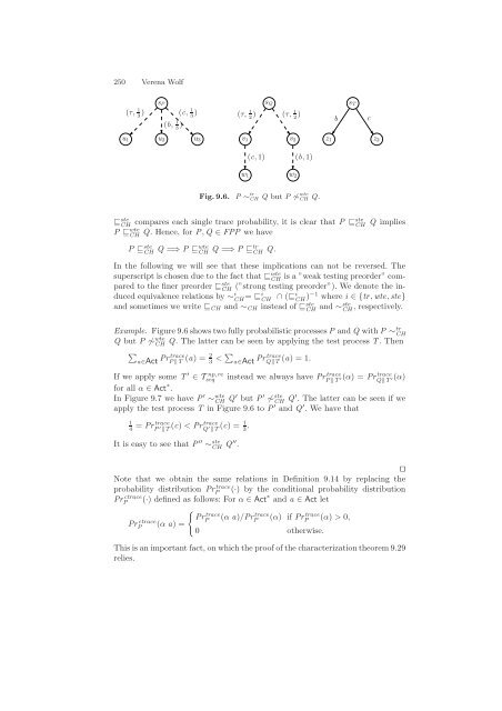
- Page 247: 248 Verena Wolf specification proce
- Page 251 and 252: 252 Verena Wolf sP (a, 1 1 ) (a, 2
- Page 253 and 254: 254 Verena Wolf v1 u1 w1 1 2 sP λ
- Page 255 and 256: 256 Verena Wolf • P ⊑ must JY Q
- Page 257 and 258: 258 Verena Wolf u1 s M ′ 1 (a, r1
- Page 259 and 260: 260 Verena Wolf Proposition 9.22. L
- Page 261 and 262: 262 Verena Wolf Now let Q min be th
- Page 263 and 264: 264 Verena Wolf (8) (⊑BC , ⊑CH
- Page 265 and 266: 266 Verena Wolf is that an action a
- Page 267 and 268: 268 Verena Wolf can perform τ-tran
- Page 269 and 270: 270 Verena Wolf T np,re seq ⊑ tr
- Page 271 and 272: 272 Verena Wolf t2 t4 a sT t1 b b t
- Page 273 and 274: 274 Verena Wolf model test processe
- Page 275 and 276: Part III Model-Based Test Case Gene
- Page 277 and 278: Part III. Model-Based Test Case Gen
- Page 279 and 280: 282 Alexander Pretschner and Jan Ph
- Page 281 and 282: 284 Alexander Pretschner and Jan Ph
- Page 283 and 284: 286 Alexander Pretschner and Jan Ph
- Page 285 and 286: 288 Alexander Pretschner and Jan Ph
- Page 287 and 288: 290 Alexander Pretschner and Jan Ph
- Page 289 and 290: 11 Evaluating Coverage Based Testin
- Page 291 and 292: 11 Evaluating Coverage Based Testin
- Page 293 and 294: 11 Evaluating Coverage Based Testin
- Page 295 and 296: 11 Evaluating Coverage Based Testin
- Page 297 and 298: 11 Evaluating Coverage Based Testin
- Page 299 and 300:
11 Evaluating Coverage Based Testin
- Page 301 and 302:
11 Evaluating Coverage Based Testin
- Page 303 and 304:
11 Evaluating Coverage Based Testin
- Page 305 and 306:
11 Evaluating Coverage Based Testin
- Page 307 and 308:
11 Evaluating Coverage Based Testin
- Page 309 and 310:
11 Evaluating Coverage Based Testin
- Page 311 and 312:
11 Evaluating Coverage Based Testin
- Page 313 and 314:
11 Evaluating Coverage Based Testin
- Page 315 and 316:
11 Evaluating Coverage Based Testin
- Page 317 and 318:
11 Evaluating Coverage Based Testin
- Page 319 and 320:
12 Technology of Test-Case Generati
- Page 321 and 322:
12 Technology of Test-Case Generati
- Page 323 and 324:
12 Technology of Test-Case Generati
- Page 325 and 326:
Increment ∆Counter 12 Technology
- Page 327 and 328:
12 Technology of Test-Case Generati
- Page 329 and 330:
12 Technology of Test-Case Generati
- Page 331 and 332:
(12.4) ✟ nat(X ′ ) {A/0, B/X
- Page 333 and 334:
12 Technology of Test-Case Generati
- Page 335 and 336:
12 Technology of Test-Case Generati
- Page 337 and 338:
a: b: (6) α1+1−α2 α2 a: b: PC:
- Page 339 and 340:
12 Technology of Test-Case Generati
- Page 341 and 342:
12 Technology of Test-Case Generati
- Page 343 and 344:
12 Technology of Test-Case Generati
- Page 345 and 346:
12 Technology of Test-Case Generati
- Page 347 and 348:
12 Technology of Test-Case Generati
- Page 349 and 350:
12.5 Summary 12 Technology of Test-
- Page 351 and 352:
13 Real-Time and Hybrid Systems Tes
- Page 353 and 354:
Test Driver SUT 13 Real-Time and Hy
- Page 355 and 356:
13 Real-Time and Hybrid Systems Tes
- Page 357 and 358:
13 Real-Time and Hybrid Systems Tes
- Page 359 and 360:
13 Real-Time and Hybrid Systems Tes
- Page 361 and 362:
13 Real-Time and Hybrid Systems Tes
- Page 363 and 364:
13 Real-Time and Hybrid Systems Tes
- Page 365 and 366:
13 Real-Time and Hybrid Systems Tes
- Page 367 and 368:
13 Real-Time and Hybrid Systems Tes
- Page 369 and 370:
13 Real-Time and Hybrid Systems Tes
- Page 371 and 372:
13 Real-Time and Hybrid Systems Tes
- Page 373 and 374:
13 Real-Time and Hybrid Systems Tes
- Page 375 and 376:
13 Real-Time and Hybrid Systems Tes
- Page 377 and 378:
13 Real-Time and Hybrid Systems Tes
- Page 379 and 380:
fitness 13 Real-Time and Hybrid Sys
- Page 381 and 382:
13.5 Summary 13 Real-Time and Hybri
- Page 383 and 384:
13 Real-Time and Hybrid Systems Tes
- Page 385 and 386:
390 Part IV. Tools and Case Studies
- Page 387 and 388:
392 Axel Belinfante, Lars Frantzen,
- Page 389 and 390:
394 Axel Belinfante, Lars Frantzen,
- Page 391 and 392:
396 Axel Belinfante, Lars Frantzen,
- Page 393 and 394:
398 Axel Belinfante, Lars Frantzen,
- Page 395 and 396:
400 Axel Belinfante, Lars Frantzen,
- Page 397 and 398:
402 Axel Belinfante, Lars Frantzen,
- Page 399 and 400:
404 Axel Belinfante, Lars Frantzen,
- Page 401 and 402:
406 Axel Belinfante, Lars Frantzen,
- Page 403 and 404:
408 Axel Belinfante, Lars Frantzen,
- Page 405 and 406:
410 Axel Belinfante, Lars Frantzen,
- Page 407 and 408:
412 Axel Belinfante, Lars Frantzen,
- Page 409 and 410:
414 Axel Belinfante, Lars Frantzen,
- Page 411 and 412:
416 Axel Belinfante, Lars Frantzen,
- Page 413 and 414:
418 Axel Belinfante, Lars Frantzen,
- Page 415 and 416:
420 Axel Belinfante, Lars Frantzen,
- Page 417 and 418:
422 Axel Belinfante, Lars Frantzen,
- Page 419 and 420:
424 Axel Belinfante, Lars Frantzen,
- Page 421 and 422:
426 Axel Belinfante, Lars Frantzen,
- Page 423 and 424:
428 Axel Belinfante, Lars Frantzen,
- Page 425 and 426:
430 Axel Belinfante, Lars Frantzen,
- Page 427 and 428:
432 Axel Belinfante, Lars Frantzen,
- Page 429 and 430:
434 Axel Belinfante, Lars Frantzen,
- Page 431 and 432:
436 Axel Belinfante, Lars Frantzen,
- Page 433 and 434:
438 Axel Belinfante, Lars Frantzen,
- Page 435 and 436:
440 Wolfgang Prenninger, Mohammad E
- Page 437 and 438:
442 Wolfgang Prenninger, Mohammad E
- Page 439 and 440:
444 Wolfgang Prenninger, Mohammad E
- Page 441 and 442:
446 Wolfgang Prenninger, Mohammad E
- Page 443 and 444:
448 Wolfgang Prenninger, Mohammad E
- Page 445 and 446:
450 Wolfgang Prenninger, Mohammad E
- Page 447 and 448:
452 Wolfgang Prenninger, Mohammad E
- Page 449 and 450:
454 Wolfgang Prenninger, Mohammad E
- Page 451 and 452:
456 Wolfgang Prenninger, Mohammad E
- Page 453 and 454:
458 Wolfgang Prenninger, Mohammad E
- Page 455 and 456:
460 Wolfgang Prenninger, Mohammad E
- Page 457 and 458:
Part V Standardized Test Notation a
- Page 459 and 460:
466 George Din inter-operability te
- Page 461 and 462:
468 George Din • Tabular Presenta
- Page 463 and 464:
470 George Din 16.3.1 Test Building
- Page 465 and 466:
472 George Din Abstract Test System
- Page 467 and 468:
474 George Din field can be marked
- Page 469 and 470:
476 George Din • omit: the value
- Page 471 and 472:
478 George Din altstep Default() ru
- Page 473 and 474:
480 George Din alt { [] httpPort.re
- Page 475 and 476:
482 George Din • Test Management
- Page 477 and 478:
484 George Din Value Type getType()
- Page 479 and 480:
486 George Din This task is rather
- Page 481 and 482:
488 George Din hosts, of preparing
- Page 483 and 484:
490 George Din A B C D MEM = 256 MB
- Page 485 and 486:
492 George Din A hardware load moni
- Page 487 and 488:
494 George Din ptcType2 ptcType3
- Page 489 and 490:
496 George Din communicate with the
- Page 491 and 492:
498 Zhen Ru Dai U2TP document is no
- Page 493 and 494:
500 Zhen Ru Dai state machines, sta
- Page 495 and 496:
502 Zhen Ru Dai TestResult TestCase
- Page 497 and 498:
504 Zhen Ru Dai can be mapped to JU
- Page 499 and 500:
506 Zhen Ru Dai 17.4 Test Developme
- Page 501 and 502:
508 Zhen Ru Dai Slave: Master: SRI
- Page 503 and 504:
510 Zhen Ru Dai sa: Slave− Appli
- Page 505 and 506:
512 Zhen Ru Dai sdConnect_To_Master
- Page 507 and 508:
514 Zhen Ru Dai BluetoothUnitTest
- Page 509 and 510:
516 Zhen Ru Dai is returned to the
- Page 511 and 512:
518 Zhen Ru Dai (1) /* test configu
- Page 513 and 514:
520 Zhen Ru Dai (1) /* test case */
- Page 515 and 516:
Part VI Beyond Testing This last pa
- Page 517 and 518:
526 Séverine Colin and Leonardo Ma
- Page 519 and 520:
528 Séverine Colin and Leonardo Ma
- Page 521 and 522:
530 Séverine Colin and Leonardo Ma
- Page 523 and 524:
532 Séverine Colin and Leonardo Ma
- Page 525 and 526:
534 Séverine Colin and Leonardo Ma
- Page 527 and 528:
536 Séverine Colin and Leonardo Ma
- Page 529 and 530:
538 Séverine Colin and Leonardo Ma
- Page 531 and 532:
540 Séverine Colin and Leonardo Ma
- Page 533 and 534:
542 Séverine Colin and Leonardo Ma
- Page 535 and 536:
544 Séverine Colin and Leonardo Ma
- Page 537 and 538:
546 Séverine Colin and Leonardo Ma
- Page 539 and 540:
548 Séverine Colin and Leonardo Ma
- Page 541 and 542:
550 Séverine Colin and Leonardo Ma
- Page 543 and 544:
552 Séverine Colin and Leonardo Ma
- Page 545 and 546:
554 Séverine Colin and Leonardo Ma
- Page 547 and 548:
19 Model Checking Therese Berg 1 an
- Page 549 and 550:
19 Model Checking 559 The first sta
- Page 551 and 552:
19 Model Checking 561 function I :
- Page 553 and 554:
coffee coin tea 19 Model Checking 5
- Page 555 and 556:
AX (φ) :=¬EX (¬φ) AF (φ) :=Atr
- Page 557 and 558:
19 Model Checking 567 Another appro
- Page 559 and 560:
19 Model Checking 569 has a transit
- Page 561 and 562:
19 Model Checking 571 The alternati
- Page 563 and 564:
19 Model Checking 573 Obviously the
- Page 565 and 566:
19 Model Checking 575 purposes ther
- Page 567 and 568:
19 Model Checking 577 otherwise it
- Page 569 and 570:
19 Model Checking 579 Expanding a P
- Page 571 and 572:
19 Model Checking 581 We conduct an
- Page 573 and 574:
• SA ⊆ Σ ∗ is a nonempty fin
- Page 575 and 576:
19 Model Checking 585 When OT is cl
- Page 577 and 578:
19 Model Checking 587 • se = s
- Page 579 and 580:
19 Model Checking 589 the new colum
- Page 581 and 582:
19 Model Checking 591 Henceforth th
- Page 583 and 584:
19 Model Checking 593 DT , the tran
- Page 585 and 586:
19 Model Checking 595 queries. At t
- Page 587 and 588:
19 Model Checking 597 Assistant 4.
- Page 589 and 590:
19 Model Checking 599 have created
- Page 591 and 592:
19 Model Checking 601 Logic (see Se
- Page 593 and 594:
19 Model Checking 603 linear time l
- Page 595 and 596:
20 Model-Based Testing - A Glossary
- Page 597 and 598:
20 Model-Based Testing - A Glossary
- Page 599 and 600:
612 Bengt Jonsson a/0 b/0 b/1 s2 s4
- Page 601 and 602:
614 Bengt Jonsson of input symbols
- Page 603 and 604:
616 Joost-Pieter Katoen The followi
- Page 605 and 606:
618 Literature [AFH94] Rajeev Alur,
- Page 607 and 608:
620 Literature [BCMD90] J. R. Burch
- Page 609 and 610:
622 Literature [BRV95] Ed Brinksma,
- Page 611 and 612:
624 Literature [CL97a] Duncan Clark
- Page 613 and 614:
626 Literature [DGNP04] Z. R. Dai,
- Page 615 and 616:
628 Literature [FHP02] Eitan Farchi
- Page 617 and 618:
630 Literature [GL02] Hubert Garave
- Page 619 and 620:
632 Literature [Hib61] Thomas N. Hi
- Page 621 and 622:
634 Literature [HR01b] Klaus Havelu
- Page 623 and 624:
636 Literature [KKL + 01] M. Kim, S
- Page 625 and 626:
638 Literature [LPY97] Kim Guldstra
- Page 627 and 628:
640 Literature [Müh97] H. Mühlenb
- Page 629 and 630:
642 Literature [Pha93] M. Phalippou
- Page 631 and 632:
644 Literature [RdBJ00] V. Rusu, L.
- Page 633 and 634:
646 Literature [Sch00] Johann M. Sc
- Page 635 and 636:
648 Literature [SVG02] S. Schulz an
- Page 637 and 638:
650 Literature [Vas73] M. P. Vasile
- Page 639 and 640:
Index =⇒ , 175 ioco, 187 ioconf,
- Page 641 and 642:
homing sequence, 8 - adaptive, 8, 2
- Page 643 and 644:
eset sequence, see synchronizing se
- Page 645:
timed transition system, 223, 360,