The ITER toroidal field model coil project

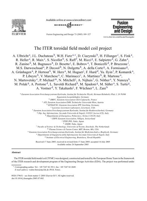
Fusion Engineering and Design 73 (2005) 189–327 

The ITER toroidal field model coil project 

A. Ulbricht a , J.L. Duchateau b , W.H. Fietz a,∗ , D. Ciazynski b , H. Fillunger c , S. Fink a , 

R. Heller a , R. Maix c , S. Nicollet b , S. Raff f , M. Ricci g , E. Salpietro d , G. Zahn a , 

R. Zanino h , M. Bagnasco h , D. Besette j , E. Bobrov a , T. Bonicelli d , P. Bruzzone i , 

M.S. Darweschsad a , P. Decool b , N. Dolgetta b , A. della Corte g , A. Formisano g , 

A. Grünhagen n , P. Hertout b , W. Herz a , M. Huguet j , F. Hurd d , Yu. Ilyin l , P. Komarek a , 

P. Libeyre b , V. Marchese a , C. Marinucci i , A. Martinez b , R. Martone o , 

N. Martovetsky e , P. Michael m , N. Mitchell j , A. Nijhuis l ,G.Nöther a , Y. Nunoya k , 

M. Polak p , A. Portone d , L. Savoldi Richard h , M. Spadoni g ,M.Süßer a ,S.Turtú g , 

A. Vostner d , Y. Takahashi j ,F.Wüchner a , L. Zani b 

Abstract 

a Euratom Association Forschungszentrum Karlsruhe, Institut für Technische Physik, Herman-Helmholtz-Platz 1, D-76366 

Eggenstein-Leopoldshafen, Germany 

b DRFC, Euratom Association CEA Cadarache, France 

c ATI, Euratom Association ÖAW, Technische Universität Wien, Austria 

d EFDA/CSU, Euratom Association IPP, Garching, Germany 

e Lawrence Livermore Laboratory, Livermore, USA 

f Euratom Association Forschungszentrum Karlsruhe, Institut für Reaktorsicherheit, Germany 

g Dip. Ing. Informazione, Seconda Università di Napoli, I-81031 Aversa (CE), Italy 

h Dipartimento di Energetica, Politecnico, Torino I-10129, Italy 

i CRPP, Euratom Association, Villigen, Switzerland 

j ITER JWS, Naka, Japan 

k JAERI, Naka, Japan 

l Faculty of Science & Technology, University of Twente, Enschede, The Netherlands 

m Plasma Science & Fusion Center, MIT, Boston, MA, USA 

n Euratom Association Forschungszentrum Karlsruhe, Institut für Medizintechnik u. Biophysik, Germany 

o Dipartimento di Ingegneria della Informazione Seconda Università di Napoli, Italy 

p Institute of Electrical Engineering, Bratislava, Slovak Republic 

Received 17 June 2005; received in revised form 17 June 2005; accepted 14 July 2005 

Available online 26 September 2005 

The ITER toroidal field model coil (TFMC) was designed, constructed and tested by the European Home Team in the framework 

of the ITER research and development program of the Engineering Design Activities (EDA). The project was performed under 

∗ Corresponding author. Tel.: +49 7247 82 3911; fax: +49 7247 82 2849. 

E-mail address: walter.fietz@itp.fzk.de (W.H. Fietz). 

0920-3796/$ – see front matter © 2005 Elsevier B.V. All rights reserved. 

doi:10.1016/j.fusengdes.2005.07.002

190 A. Ulbricht et al. / Fusion Engineering and Design 73 (2005) 189–327 

the leadership of European Fusion Development Activity/Close Support Unit (EFDA/CSU), Garching, in collaboration with the 

European superconductor laboratories and the European industry. The TFMC was developed and constructed in collaboration 

with the European industry consortium (AGAN) and Europa Metalli LMI supplied the conductor. The TFMC was tested in the 

test phase I as single coil and in phase II in the background field of the EURATOM LCT coil in the TOSKA facility of the 

Forschungszentrum Karlsruhe. In phase I, the TFMC achieved an ITER TF coil relevant current of about 80 kA and further 

representative test results before the end of the EDA. In the more complex test phase II, the coil was exposed to ITER TF 

coil relevant mechanical stresses in the winding pack and case. The tests confirmed that engineering design principles and 

manufacturing procedures are sound and suitable for the ITER TF full size coils. The electromagnetic, thermo hydraulic and 

mechanical operation parameters agree well with predictions. The achieved Lorentz force on the conductor was about 800 kN/m. 

That has been equivalent to the Lorentz forces in ITER TF coils. 

© 2005 Elsevier B.V. All rights reserved. 

Keywords: ITER; TFMC; EDA 

1. Introduction 

The oil crises in the beginning of the 1970’s 

stimulated the research for energy sources outside the 

combustion of coal and natural gas. Besides nuclear fission, 

which was already an available energy source, the 

magnetic confinement for the controlled fusion reaction 

has been looked on as a promising energy source 

for the future with an inexhaustible fuel source. The 

first conceptual designs of fusion reactors of the tokamak 

type were developed [1]. The dimensions of their 

large magnet systems showed soon that the magnets 

have had to be superconducting if the reactor should 

have a positive energy balance. Since the next generation 

of large plasma physics experiments (JET, TFTR, 

JT-60) were planned at that time with normal conducting 

magnets the necessity was recognised that, in 

parallel, the development of superconducting magnet 

technology for such types of magnets is indispensable. 

A technology experiment for the toroidal field coil system 

of the tokamak magnet system was initiated under 

the auspices of the International Energy Agency (IEA). 

This was the construction and test of a superconducting 

six-coil torus (Large Coil Task, LCT), with coil technology 

scalable to reactor coils, within an international 

collaboration of EURATOM, European Community; 

JAERI, Japan; SIN/BBC, Switzerland; ORNL, USA 

[2]. The LCT was successfully completed in 1987. 

In that project various forced-flow-cooled conductor 

concepts as well as basic design principles and components 

for large superconducting coils were developed 

and tested. In 1983, the NET team was established in 

Garching (Germany) with the aim to coordinate the 

European fusion activities and to develop a European 

design of a device to be built after JET [3,4]. 

The NET design has clearly demonstrated the need 

of high magnetic field (Nb3Sn) and high current carrying 

conductors; therefore, cables in conduit with 

forced-flow-cooled conductors has been the choice for 

application in the future. Several Nb3Sn and NbTi conductors 

were fabricated in short lengths and tested 

successfully in the SULTAN facility (Switzerland) 

[5]. 

In two medium size experiments POLO at Research 

Center Karlsruhe, Germany, in collaboration with CEA 

Cadarache, France, and DPC JAERI, Japan, in collaboration 

with MIT, USA, the superconducting technology 

for the poloidal field tokamak coils that had to withstand 

higher magnetic field transients and electrical 

losses than the TF coils, were successfully developed 

[6–9]. In addition, the necessary high voltage technology 

that has been indispensable for handling the tens of 

GJ of stored energy in large superconducting magnet 

systems, was developed in the POLO project [10]. 

Simultaneously with the developments of large 

superconducting tokamak magnets several medium 

size tokamaks with superconducting toroidal field 

coils for plasma physics experiments were constructed 

and successfully operated (T10, T15 [11], 

TORE SUPRA [12], TRIAM-1M [13]). The reliable 

operation of the medium size superconducting 

tokamaks has contributed to convincing 

the plasma physics community of the advantages 

and reliability of superconducting magnet technology.

The application and continuation of these developments 

were initiated by the ITER Conceptual (CDA) 

and Engineering Design Activity (EDA) in the 1990s. 

There were no more doubts that the ITER magnet 

system had to be constructed with superconducting 

coils [14]. In the beginning of the EDA in 1992, this 

led to the superconducting model coils of the ITER 

magnet system in the ITER research and development 

program. It was decided to construct and test a central 

solenoid model coil (CSMC) and a toroidal field 

model coil (TFMC). The necessary magnetic field levels 

between 11 and 13 T required use of the strain 

sensitive Nb3Sn as the superconducting material and 

this was a great challenge for the conductor and winding 

fabrication technology [15]. This resulted in the 

development of new structural materials that had to 

be compatible with the heat treatment and modified 

construction principles of the winding pack and coil 

structure. All that needed the confirmation in an overall 

test, which was covered by the ITER model coil 

program. 

The CSMC was constructed and tested by the ITER 

partners Japan, Russian Federation, USA, and European 

Union in JAERI, Naka (Japan) [16]. 

The TFMC was constructed by the European Union 

alone and tested in FZK Karlsruhe (Germany) with the 

participation of the ITER partners. 

Both tests were successfully completed in 2002. 

The CSMC project was concluded with the test of 

two three insert coils [17]. The first one was JAERI’s 

CS conductor insert coil (CSCI) followed by RF’s 

TFCI (TF conductor insert coil) demonstrating the 

pulse field capability of the ITER conductor concepts 

[18]. The third one was the JAERI’s ALI 

(Nb3Al conductor insert coil), an alternative material 

to Nb3Sn but with a more sophisticated fabrication 

technology [19]. In test Phase 1 (2001), the 

TFMC achieved with 80 kA the highest current in 

a large superconducting coil [20] and in test Phase 

2, ITER TF coil equivalent Lorentz forces of about 

800 MN/m. 

The subject of this contribution is an overview of 

the TFMC project within the European Union with the 

international ITER collaboration. The main features 

of design, construction of the TFMC and finally the 

TFMC test results in the TOSKA facility are described 

to guide the interested reader in more detailed publications 

of different areas. 

A. Ulbricht et al. / Fusion Engineering and Design 73 (2005) 189–327 191 

2. Project objectives and management 

The ITER design foresees to use for the TF coils 

aNb3Sn cable in a circular thin walled conduit, insulated 

and completely enclosed in a groove in steel plates 

[21]. These are then stacked together to form the winding 

pack and supported by a steel case. The concept 

is demonstrated by two large industrial actions. The 

first one is the fabrication of a racetrack shaped model 

coil (TFMC), with outer dimensions of 2.8 m × 3.9 m, a 

peak field of 9.97 T (in pancake 2.2 in the 80/16 kA load 

case, 8.8 T in the 70/16 kA load case) and a total number 

of Ampere turns of 7.84 MA (6.86 MA for 70 kA) 

including an overall test. The second one is the fabrication 

of two full size sections of a case and a radial 

plate [22,23]. The racetrack shape for the TFMC was 

selected simplifying the fabrication and reducing the 

costs. The bending free D-shape is a specific property 

of the torus operation, which has no importance in a 

two coil test configuration. On the other hand, relevant 

stress levels (radial pressure, shear stresses) and 

Lorentz body forces on the conductor comparable to 

those of the full size ITER TF coils were achieved by 

this configuration (see Section 8). The specific problems 

of the fabrication of full size TF coils (radial plates 

and case components) was assigned in the second task 

mentioned before. 

The objectives of the TFMC are as follows: 

(a) To develop and verify the full scale TF coil manufacturing 

techniques, in particular the following 

features: 

- plate manufacturing (forming the grooves); 

- fitting the conductor in the groove after heat 

treatment and insulation (i.e., predictable geometry 

change); 

- closing the groove with a cover plate and plate 

insulation; 

- fitting the winding into the case, gap filling and 

case closure. 

(b) To establish realistic manufacturing tolerances. 

(c) To bench-mark methods for the ITER TF coil 

acceptance tests, including insulation and impregnation 

process monitoring, welding quality of closure 

welds for cover plates and case, and conductor 

joint electrical quality. 

(d) To gain information on the coil’s mechanical 

behaviour, operating margins and in-service mon-


itoring techniques, particularly for the insulation 

quality. 

The TFMC and its test arrangement were designed 

to be representative for the ITER TF coil in respect of 

layout and electrical and mechanical stresses [24–27]. 

The layout of the TFMC overtook as many as possible 

features of the ITER TF coil design on a scale 

nearly 1:1. Only the overall dimensions had to be chosen 

in a way that the TFMC assembled together with 

the already existing EURATOM LCT coil fitted into 

the TOSKA facility of the FZK/ITP at Karlsruhe [28]. 

The construction and test of the TFMC was the 

main part of one of the seven large R&D projects of 

the ITER EDA [29]. The TFMC has been conceptually 

designed by the EURATOM Associations CEA 

Cadarache, ENEA Frascati and Forschungszentrum 

Karlsruhe (ITP) under the coordination of EFDA-CSU 

Garching (the former NET Team). The work sharing 

between the laboratories was adapted according to their 

experimental facilities as well as their expertise in the 

different fields and special skills for assistance during 

the construction and the preparations for the test [20]. 

A consortium of European companies, called 

AGAN (Accel, Alstom, Ansaldo, Noell) developed and 

performed the engineering design and manufacture of 

the TFMC under the surveillance of the EFDA-CSU 

Garching on behalf of EURATOM, in tight collaboration 

with the mentioned associations. The conductor 

was manufactured by Europa Metalli in separate contract 

and provided by EFDA-CSU to the AGAN consortium. 

The work sharing within AGAN was as follows: 

Accel Instruments: Design calculations, technical 

project and quality management. 

Alstom: Winding pack assembly, manufacturing of 

coil case and superconducting bus bars, final coil 

assembly and instrumentation. 

Ansaldo Superconduttori: Double pancake module 

fabrication. 

Babcock Noell Nuclear: Design calculations, commercial 

management, structural components (radial 

plates, intercoil structure), related instrumentation, 

and assembly of the test configuration at TOSKA site. 

The TFMC construction phase was accompanied by 

seven review meetings over 5 years within the international 

ITER collaboration. 

The test of the TFMC was conducted by the Coordination 

Group consisting of the EU project manager 

as chairman, delegates of the ITER partners, ITER 

International Team and the test-hosting laboratory. The 

Group was supported by two experts groups (Test & 

Analysis and Operation Group), consisting of association 

staff, which prepared, performed and evaluated 

the test. 

The testing in TOSKA facility at FZK Karlsruhe was 

supported by participation of scientists representing all 

ITER partners (EU, JA, RF, US) and ITER central team. 

3. Toroidal field model coil layout and 

manufacture 

3.1. Layout of the TF model coil 

3.1.1. TFMC Project objectives and layout 

The special coil design (Fig. 3.1) with a circular 

Nb3Sn cable in conduit conductor placed into the spiral 

grooves of the 316LN stainless steel (SS) radial 

plates required the development of new manufacturing 

methods including the associated tooling. This has 

been described in several publications [30–34]. The 

design, manufacture and quality assurance (QA) results 

are described in detail in [35]. 

The ITER TF Model Coil design parameters and the 

main operating data are shown in Tables 3.1 and 3.2 in 

comparison with the ITER TF coils. 

Table 3.1 

ITER TF model coil design parameters 

Properties ITER TF TFMC 

Conductor diameter [mm] 43.4 40.7 

Nominal turn insulation 

thickness [mm] 

1.25–2.0 2.5 

Nominal DP module 

insulation 

1.0 1.5 

Total insulation between 

DP modules [mm] 

∼5.0 ∼4.0 

Ground insulation 

thickness [mm] 

8 8 

Number of DP modules 7 5 

Total number of turns 134 98 

Winding min. radius [mm] 500 600 

Case thickness [mm] 75–240 70–80 

Overall dimensions [m] 14.7 × 8.5 × 1.4 3.8 × 2.7 × 0.77 

Mass per coil [t] ∼340 ∼40

3.2. Conductor manufacture 

3.2.1. Strand 

A total of 3.9 t of internal tin Nb3Sn strand (ITER 

HP1 specifications) have been used to fabricate about 

900 m of conductor for the five double pancakes of 

the TFMC by the Europa Metalli Company. The production 

has demonstrated good reproducibility of the 

conductor performance. Table 3.3 shows the main 


Fig. 3.1. Layout of the TF model coil (TFMC). 

parameters of the TFMC Nb3Sn filamentary strand 

(Fig. 3.2) and the NbTi filamentary strand of the bus 

bars. 

3.2.2. Cable 

The cable, composed of 1080 wires one-third of 

which are Cu wires, has a 304 stainless steel central spiral, 

and an Inconel wrap for the last-but-one cable stage 

(10% gap) and for the final cable (half overlapped). The


Table 3.2 

Main operating data of the TFMC in comparison with the ITER TF 

coils 

Operating data ITER TF TFMC alone/ 

TFMC + (LCT) 

Operating current (LCT) 

[kA] 

68 80/80(16) 

Ampere turns (LCT) [MA] 9.1 7.8/7.8 (9.4) 

Bmax in ITER TF/TFMC [T] 11.8 7.78/9.97 

Max. compression stresses 

on coil [MPa] 

−130 −/−180 

Max. inter-DP shear stresses 

[MPa] 

30 −/50 

Max. Tresca stresses in case 

[MPa] 

527 −/470 

Max. Lorentz force [kN/m] 780 622/797 

cable build-up and the cross-section of the conductor 

are shown in Fig. 3.3 with the main parameters listed 

in Table 3.4. 

3.2.3. Jacket and jacketing 

Seamless 316LN SS tubes, with 1.6 mm wall thickness, 

were butt-welded to the final unit length (TIG 

orbital welding). After pulling the cable into the jacket 

the conductor was brought to the final specified dimensions 

by a set of rollers and calendered onto a 2.5 m 

diameter drum. 

The manufacturing process has shown the importance 

of maintaining proper tuning of the cabling system 

as one cable had a slight undulation causing difficulties 

during introduction into the jacket. It also turned 

out that the use of a center spiral of a different supplier 

Table 3.3 

Main parameters of the strands for the TFMC conductor and the bus 

bars 

Properties TFMC Bus bar 

Sc. material Nb3Sn NbTi 

Diameter [mm] 0.810 ± 0.003 0.810 ± 0.003 

Twist pitch [mm] ≤10 ≤10 

Twist direction RHHa RHHa Cu/nonCu ratio 1.50 ± 0.05 2.4 ± 0.05 

Barrier 2 �m Cr coating 10 �m CuNi int. 

barrier 

Average IC 153 A at 12 T and 4.2 K 440 A at 5 T and 

4.2 K 

RRR >100 >120 

a Right hand helix. 

caused a significant change in the flow resistance (Section 

6.2.1). 

The conductor design and manufacture has been 

described in several publications [36,37]. 

The NbTi bus bar conductor was fabricated according 

to a similar method. Instead of a tube a thick-walled 

stainless steel jacket (316LN) was used developed for 

the central solenoid conductor within a task of the European 

Fusion Technology Program. 

3.3. Double pancake (DP) module manufacturing 

3.3.1. Pancake winding 

An automatically controlled calendering system 

was built and integrated into the winding line consisting 

of a roll-off jack, guiding rollers, straightening 

unit, cleaning and sand blasting unit, and calendering 

device. Stainless steel plates with spiral grooves served 

as winding templates, reaction moulds and references 

to position the conductor terminations. 

During winding (Fig. 3.4), the conductor diameter 

was reduced from 40.9 mm on the spool to about 

40.5 mm after straightening and further to an oval shape 

of 40.4 ± 0.1 mm in the curved regions of the racetrack. 

The as built TFMC double pancake data are listed in 

Table 3.5. 

3.3.2. Manufacturing of the terminations 

The terminations consist of an explosion bonded 

copper/stainless steel box, in which the cable ends were 

pressed by a cover with a force of about 2 MN. The 

Inconel over-wrap of the cable, the surface section of 

the petal wrap and the Cr-coating of the strands were 

removed before inserting the cable ends into the box. 

The cover was fixed by TIG welding and kept in a rigid 

tool fixed to the reaction mould during the whole heat 

treatment cycle. This type of terminations developed by 

CEA was qualified with full-size joint samples (FSJS) 

showing very low resistance as described in Section 7 

[38,39]. A cross-section of such a termination is shown 

in Fig. 3.5. 

3.3.3. Reaction heat treatment 

The reaction heat treatment (210 ◦ C/100 h, 

340 ◦ C/24 h, 450 ◦ C/24 h, 650 ◦ C/200 h) was performed 

in a special oven using high purity Argon as an 

inert gas flowing inside the conductor and with slight 

overpressure in the oven (Fig. 3.6). Some of the heat


Fig. 3.2. Cross-section of the Europa Metalli Nb3Sn internal tin strand. 

Fig. 3.3. Cross-section and build-up of the TFMC conductor.


Table 3.4 

Parameters of the TFMC and bus bar conductor 

Properties TFMC Bus bar 

Cable build-up (see Fig. 3.3) (2sc+1Cu)× 3 × 5 × 4 × 6 (MC2) 3 × 4 × 4 × 4 × 6 

Cabling direction at all stages Right hand Right hand 

No. of s/c strands 720 1152 

No. of Cu strands 360 0 

Central tube diameter 12.0 mm × 1.0 mm 12.0 mm × 1.0 mm 

Central spiral gap 35 and 50% 50% 

Wrapping of last-but-one stage 0.1 mm thick Inconel tape; gap 10% 0.1 mm thick Inconel tape; gap 10% 

Wrapping of last stage 0.1 mm thick Inconel tape; half overlapped 0.1 mm thick Inconel tape; half overlapped 

Compacted cable diameter 37.4 mm 38.2 mm 

Jacket material 316 LN 316 LN 

Conductor dimensions 

Twist pitches [mm] 

40.7 mm circular 51 mm square 

Stage 1 (first triplet) 45 ± 5 45± 5 

Stage 2 85 ± 5 85± 5 

Stage 3 125 ± 5 125 ± 5 

Stage 4 (LBO, last-but-one) 160 ± 10 160 ± 10 

Stage 5 (full size) 400–425 400–425 

treatments were interrupted due to oven failures, and 

were continued after repairs. Witness strands reacted 

with the pancakes showed no degradation. 

During heat treatment the conductor expanded in 

length by about 0.05%. This was overcome by increasing 

the width of the groove of the reaction mould 

leaving the conductor some freedom to move. 

After heat treatment a dimensional check and leak 

test were carried out on all pancakes. All the pancakes 

including terminations were leak tight to better than 

1 × 10 −10 mbar l/s. 

Fig. 3.4. Winding of a pancake into a reaction mould. 

3.3.4. Turn insulation and transfer 

The pancakes were spread in a fixture that ensured 

that the reacted conductor was not strained more than 

0.2%. In this position, the glass–Kapton turn insulation 

and the co-wound voltage taps were applied manually 

as shown in Fig. 3.7. Subsequently, the pancake was 

transferred into the grooves of the radial plate using 

reference marks on conductor and plate. The turns were 

held in the grooves by covers spot welded in ∼200 mm 

distances. After turning the plate over the second pancake 

of a DP module was transferred in the same way. 

Fig. 3.5. Cross-section of a conductor termination. The terminations 

of two adjacent pancakes were soft soldered (inner pancake and winding 

end joints) or electron beam welded (outer pancake joints) and 

finally clamped together.

Table 3.5 

TFMC double pancake data as fabricated 

Properties Specified DP1 DP2 DP3 DP4 DP5 

Length of pancakes 1/2 [m] 73/83 83/83 83/83 83/83 83/73 

No. of turns in pancake 1/2 

Average conductor dimensions of pancake 

9/10 10/10 10/10 10/10 10/9 

Straight [mm] 40.7 × 40.7 40.3 × 40.4 40.3 × 40.4 40.5 × 40.5 40.5 × 40.5 40.5 × 40.5 

Bent [mm] 

Local void fraction calculated for pancake 

40.3 × 40.4 40.0 × 40.2 40.4 × 40.2 40.4 × 40.3 40.5 × 40.3 

Straight [%] 35.4% 34.1 34.1 34.7 34.7 34.7 

Bent [%] 

Last cabling pitch in termination 

Pancake 1 

34.1 33.4 34.0 34.0 34.3 

Innera [mm] 435 440 425 440 435 

Outera [mm] 

Pancake 2 

440 430 435 445 440 

Innera [mm] 440 445 440 435 440 

Outera [mm] 435 440 440 432 440 

Terminations void fraction calculated [%] ∼23 ∼23 ∼23 ∼23 ∼23 

Central tube in the terminations [mm × mm] 12 × 3 12× 3 12× 3 12× 3 12× 3 12× 3 

Heat treatment and incidents 100 h, 210 ◦ C; 24 h, 340 ◦ C; 

24 h, 450 ◦ C; 200 h, 650 ◦ C 

a Termination. 

Interrupted due to 

oven failure at 

340 ◦ C 

Interrupted due to 

oven failure at 

340 ◦ C 

Ok; none Interrupted due 

to oven failure 

at 340 ◦ C 

Ok; none 

A. Ulbricht et al. / Fusion Engineering and Design 73 (2005) 189–327 197


Fig. 3.6. Two pancakes in the reaction moulds in front of the furnace. 

The radial plates (RP) and covers are made of 316LN 

stainless steel by forging and machining. Thanks 

to intermediate heat treatments at 950 ◦ C the flatness 

of the finally machined radial plates was within 

∼0.2 mm distinctly better than originally expected by 

industry. 

Fig. 3.7. Insulation of the turns including the installation of the cowound 

stainless steel tape voltage taps and transfer into the grooves 

of the radial plate. 

3.3.5. Soldering and clamping of the inner joints 

It turned out that after heat treatment and removal 

of the fixture all terminations deformed into a bananalike 

shape, the copper sole being on the convex side. 

This posed some problems in the assembly of the 

terminations into the inter-pancake joints, but has 

been solved by precise machining of the two adjacent 

copper soles before connecting them. Because 

the necessity of such a machining was expected, some 

extra copper thickness was provided. The resulting 

joints were in agreement with the expectations (see 

Section 7). 

The procedure to soft-solder the inner terminations 

to form the inter-pancake joint caused a 2 mm thermal 

expansion, which was taken up by the not yet 

impregnated turn insulation. After soldering, the joints 

were fitted with rigid clamps as shown schematically 

in Fig. 3.5. 

3.3.6. Laser welding of the covers 

To give the DP modules the right stiffness, the covers 

had to be welded with a penetration of 2.5 mm. 

Nd–YAG laser welding (2 kW/(0.6 m min), automatic 

tracking) was chosen to keep the heat input at a 

minimum (Fig. 3.8). Optimum flatness of the DP 

modules of less than 2 mm was achieved by several 

turnovers of the plate during the operation. With 

an eddy current test method developed by ENEA it 

was possible to check the weld quality and penetration. 

Fig. 3.8. Laser welding of the covers onto the conductor grooves of 

the radial plate with automatic tracker system.

3.3.7. Module ground insulation and impregnation 

The modules were wrapped by 1.3 mm glass/Kapton 

insulation followed by an impregnation with DGEBA 

epoxy resin at about 75 ◦ C followed by a curing cycle at 

about 125 ◦ C. The resin could penetrate through holes 

in the covers into the turn insulation. Some of the good 

flatness of the radial plates was lost due to a too low 

stiffness of the impregnation mould. 

3.3.8. Final tests on the DP modules 

Before shipment, all DP modules passed insulation 

resistance tests (500 V DC conductor to radial plate), 

dielectric test (3 kV DC and ACpeak-to-peak conductor to 

radial plate and 1.5 kV DC radial plate to ground), continuity 

and mutual insulating test on all voltage taps, gas 

flow test and a leak test at 30 bar helium internal pressure 

in a vacuum vessel to a level of 1 × 10 −10 mbar l/s. 

The test results are compiled in Table 3.6. 

3.4. Winding pack manufacture 

3.4.1. DP stacking and winding pack impregnation 

A special stacking device was developed to align 

and stack the DP’s to form the winding pack, as shown 

in Fig. 3.9. Glass felt was introduced between the DP 

modules in order to get good impregnation and bonding 

between the DP’s and to adjust the height of the winding 

pack. During impregnation with epoxy resin a further 

setting of the glass felt took place, namely between 

the higher compressed lower DP’s. The total height of 


Fig. 3.9. Stacking of the DP modules with glass felt inter layer to 

equalize tolerances and to adjust the height of the winding pack. 

the winding pack was decreased by about 2 mm. The 

impregnated winding pack can be seen in Fig. 3.10. 

3.4.2. Outer joint manufacturing 

The gap between adjacent terminations had to be 

bridged by copper shims to secure a good contact. 

Unlike the inner joints, it was not possible to connect 

the terminations of two adjacent double pancakes 

by soldering because of the 2 mm thermal expansion 

during heating. This would have caused unacceptably 

high stresses in the jacket. 

These two technical constraints led the supplier to a 

solution using copper pins as shims (9–10 mm diameter) 

that were introduced into holes drilled between two 

Table 3.6 

Data of final tests of the DP modules at Ansaldo works 

Flow test Pressure 

drop [bar] 

DP1 [N m3 /h] DP2 [N m3 /h] DP3 [N m3 /h] DP4 [N m3 /h] DP5 [N m3 /h] 

N2 mass flow through pancake 

DPX.1 (X = 1–5) 

N2 mass flow through pancake 

DPX.2 (X = 1–5) 

High voltage tests 

3 kV DC between turns and 

RP, 1 min [G�] 

3kVpeak–peak AC between 

turns and RP, 1 min [mA] 

1.5 kV DC between RP and 

ground, 1 min [G�] 

2 11.5 9.7 10.0 9.4 11.5 

4 21.0 18.3 18.7 17.5 21.0 

2 11.5 9.0 10.2 9.5 11.0 

4 21.0 16.5 18.9 17.0 20.0 

13 9.2 8.35 7.6 7.75 

91 99 102 101 92 

9.7 9.5 3 10 10.9


Fig. 3.10. The impregnated winding pack. The Helium outlet tubes 

protrude and the outer joint area is still left free. 

adjacent terminations and protruding into both copper 

soles. These pins were electron beam welded in such 

a way that the bulk temperature of the terminations 

did not reach more than 60 ◦ C. This method has been 

validated with a full-size joint sample as described in 

Section 7. 

3.4.3. Ground insulation and impregnation 

After having provided the outer joints with welded 

clamps of aluminium alloy they were wrapped by 

the required sliding layer (Tedlar tape) and a combined 

glass–Kapton insulation. Then 8 mm of combined 

glass–Kapton insulation was built up on the 

whole surface in order to form the ground insulation, 

which was then impregnated with DGEBA epoxy resin. 

After impregnation and before assembly with the 

coil case dielectric tests (10 kV DC and ACpeak-to-peak) 

and flow/pressure/leak tests were performed successfully. 

3.4.4. Stainless steel case 

The case of the TFMC was made of 70–90 mm thick 

316LN stainless steel sheet. The thickness was defined 

after FE calculations for the worst load case. 

The pieces were MAG welded together by qualified 

procedures to a U-shaped structure. All welds were 

ultrasonically tested. Defects had to be repaired, which 

were unacceptable according standards for highly 

loaded austenitic welds. 

The tightly toleranced shape was obtained by 

machining and local heating, partially in combination 

with the applied force of hydraulic jacks. 

Fig. 3.11. The winding pack in the stainless steel case. After filling 

the gap between the two with silica sand the cover was placed on top 

and subsequently welded. 

The welding chamfers on top of the U-shape and 

on the cover plate were copy milled. A fit within a few 

tenth of mm was achieved. 

3.4.5. Winding pack/case assembly 

For the winding pack/case assembly, both were 

in reversed position (i.e., bottom up). After having 

brought up the glass felt layers on the bottom of the 

winding pack the case was put on. A special tool fixed 

the assembly and allowed a turn over without slipping 

out of place. 

After having the gap filled with silica sand and placing 

glass felt on top, the case cover was positioned on 

top (Fig. 3.11). The first three passes of the root were 

TIG welded and inspected using dye penetrant. The 

remaining 70–90 mm deep seam was MAG welded. 

Ultrasonic testing on all welding seams was performed 

by the French Institut de Soudure. All located defects 

larger than those agreed had to be repaired, particularly 

in highly stressed areas of the case. 

After cover welding the case openings were sealed 

to make it vacuum tight for impregnation with the same 

type of epoxy resin and the same curing procedure, as 

used for the previous impregnations (see Section 3.3.7). 

For impregnation, the same mould was used again as a 

heating vessel. 

3.4.6. Final machining and surface finish 

The final machining of the interfaces and cooling 

channels on the outer circumference was done after

impregnation of the coil in the case and sand blasting 

of the outer surface. After the final machining the covers 

were welded on the cooling channels of the outer 

circumference and pressure and leak tested. The final 

surface finish was achieved by degreasing with agreed 

solvents. 

3.4.7. Headers and bus bars 

The inlet and outlet header assemblies have been 

built up on assembly frames. After having been pressure 

and leak tested they were transferred onto the 

TFMC. 

A number of sensors (strain gauges, rosettes, displacement, 

temperature, etc.) as described in Section 

3.7 were mounted onto the TFMC. The Kapton insulated 

high voltage cables have been equipped with the 

warm vacuum tight feed throughs by FZK and provided 

by industry with the cold end pieces that were 

connected with the voltage taps coming from the pancakes 

and the radial plates. 

The bus bars have been manufactured from a CS1 

type conductor using NbTi strands and a stainless steel 

square jacket. The bus bar terminations are of the same 

type as the EU FSJS’s [40,38]. 

Two types of bus bars were manufactured: Bus bars 

type 1 were mounted on the TFMC connected to the 

coil terminations (see Fig. 3.12). After assembly in the 

TOSKA facility they were connected to the terminations 

of bus bars type 2 forming part of the TOSKA 

current lead system (so-called cryostat extension). The 

busbars were insulated by multi-layer wrapping with 

glass-Mica tapes wetted with ambient temperature curing 

epoxy resin. 

3.4.8. Intermediate and final tests at suppliers 

works 

Intermediate tests (dielectric, pressure/flow/leak, 

geometrical, etc.) were performed on DP modules, 

winding pack in different stages and subassemblies. 

A final 30 bar helium internal pressure and leak test 

of the TFMC with all headers and instrumentation was 

carried out in a vacuum tank built by modifying the 

impregnation mould. The total leak rate had to be: 


Table 3.7 

TFMC Data measured at Alstom Works 

Properties Test condition Result 

Insulation resistance coil to ground 500 V DC 13 G� 

Joints/radial plates to ground 10 kV DC 1 min 10 G�) 

Impedance 3.55 kVrms AC 1 min 149 mA (∼24 k�) 

Turn insulation test up to 100 V/turn Impulse up to 9800 V Ok 

Inductance measurement on TFMC at 100 Hz 4.56 �H; Q-factor: 0.07 

at 1 kHz 153 �H; Q-factor: 0.25 

Global resistance of coil at 19 ◦C 0.0352 � I = 98.4 A/U = 3.471 V 

Instrumentation and quench detection wires All ok except: temperature sensor; TI832 and strain 

gauge rosette GRI830 

ing was qualified and tested to recognised standards. 

Subassemblies were leak tested in a special vacuum 

tank (


Fig. 3.13. TFMC flow and instrumentation scheme for winding and bus bars. 

Fig. 3.14. Voltage tap instrumentation scheme for the first double pancake DP1 as example. EDI: short (A), respectively, long voltage taps 

(including 600 mm of conductor on each side) for joint resistance measurement; EDS: voltage taps for measurement of pancake, respectively, 

double pancake voltage; EK: compensated voltage taps for diagnostic; Ja: outer pancake joint; Ji: inner pancake joint; P: pancake; QCW: 

compensated voltage for quench detection; R: ohmic resistor (for simplification the radial plate RP is directly connected across a resistor to the 

inner joint. In reality the resistor is outside the vacuum vessel at room temperature; RP: radial plate.


bonded to the ground insulation of the coil so that the 

insulation was electrically tight in case of a vacuum 

breakdown and passing through the Paschen minimum 

pressure. 

3.7.2. Temperature sensors 

Three types of temperature sensors were used to 

monitor the temperature of the coolant of the coil, 

the case and the ICS. Due to the high magnetic field 

the cheaper TVO sensors could not be used in certain 

positions. For measuring the helium temperature, 13 

CERNOX sensors (11 for the winding and 2 for the 

ICS) were placed directly in the helium flow inside 

the cooling pipes at the inlet and outlet points of the 

flow scheme. However, 31 TVO sensors were installed 

for monitoring and controlling the cool down process. 

They were positioned on the surface of the coil 

case, the surface of the ICS and on cooling pipes. 

Additional 4 Pt100 sensors were used to monitor the 

hot spots of the coil case and the ICS during cool 

down. 

3.7.3. Strain gauges, rosettes and displacement 

transducers 

The Lorentz forces deformed the overall and crosssectional 

shape of the coil case and the ICS. Thirtyfour 

individual strain gauges and 11 rosettes were 

installed to measure the surface strains at the main 

symmetry planes of TFMC, at the highly stressed 

wedges of the ICS and at the contact areas of TFMC, 

ICS and LCT. Twenty-four displacement transducers 

monitored the elongation of the joint area connecting 

adjacent double pancakes of the winding and 

the overall distortion of the shape of TFMC and the 

change of mutual position (details are presented in 

Section 8). 

3.7.4. Flow rate and pressure drop sensors 

The helium flow rate was measured by Venturi tube 

flowmeters Pancake DP1.1 and pancake DP1.2 were 

provided with individual Venturi flowmeters and pairs 

of capillaries for pressure drop measurements, because 

these were the pancakes foreseen for the heat slug injection 

to investigate the operation limits of the TFMC. 

There were another six Venturi flowmeters installed at 

the inlet points of the remaining double pancakes and 

bus bars. 

3.7.5. Magnetic field sensors 

In the geometrical center of TFMC, a pair of Hall 

probes and pick-up coils were installed to measure the 

magnetic field of the coil. 

3.7.6. Heaters at the inlet pipes of the DP’s 1.1 

and 1.2 

In order to make it possible to heat the helium flowing 

into the two pancakes adjacent to the LCT coil the 

corresponding inlet pipes were equipped with resistive 

heaters with a maximum power of 1000 W. 

3.8. Summary 

The specific manufacturing technology for the ITER 

TF coil design was successfully developed by the construction 

of the ITER TFMC. The main effort was 

put in the fabrication of the radial plates and the specific 

manufacturing technologies related to heat treatment 

and the brittleness of the Nb3Sn conductor. The 

milling of the groves as well as radial plate flatness 

within the small tolerances was a challenging task, 

which was solved. The “wind–react–insulate–transfer” 

method was the solution for handling the sensitive 

conductor without causing any degradation. Tolerance 

problems between the reacted conductor spiral 

and the groove of the radial plate were solved. All 

joints had to be fabricated with the reacted conductor. 

This was no problem with the applied joint technology. 

Soldering and EB welding techniques were 

used joining the special prepared conductor end of 

the pancakes with each other. The insulation system 

was based on fibreglass–Kapton tapes wrapping with 

a three step vacuum impregnation including the fixture 

of the winding pack in the thick-walled stainless 

steel coil case. The assembling of the TFMC 

with the inter-coil structure, which was manufactured 

by another company, was performed at the 

TOSKA site. The coil was equipped with an electrical, 

thermal-hydraulic, and mechanical instrumentation, 

which was integrated in the manufacturing steps 

of the TFMC. 

The whole manufacturing process was accompanied 

by quality assurance procedures guaranteeing the quality 

of the product in respect of its electrical, thermalhydraulics 

and mechanical properties. 

The manufacturing of the TFMC was a coordinated 

task under the leadership of EFDA between the indus-

trial consortium AGAN and the European superconducting 

magnet laboratories. 

4. TOSKA facility 

The TOSKA facility was constructed in the early 

1980s for the testing of large superconducting magnets 

for the magnetic confinement of nuclear fusion. The 

first test was the acceptance test of the LCT coil (1984) 

before shipment to the international test facility of “The 

Large Coil Task” at the Oak Ridge National Laboratory, 

USA [44,2]. After the conclusion of the test of the 

poloidal field model coil POLO (1995) [9], the cryogenic 

and electrical supply systems, the measuring and 

control equipment including data acquisition as well as 

the lifting capacity of the crane system were extended 

and modernised in the frame of a task agreement with 

ITER Director for the test of the ITER TFMC. The 

extension was performed in two steps including the 

intermediate test operation of the LCT coil with superfluid 

forced-flow helium II cooling (1996–1997) [45] 

and the acceptance test of the W 7-X DEMO coil in 

the background field of the LCT coil (1999) [46,47]. 

The TFMC was tested in 2000 as a single coil (Phase 

1) [20] and in 2002 in the background field of the LCT 

coil (Phase 2) [52]. 

4.1. Installation of the test configuration in the 

TOSKA facility 

4.1.1. Installation 

In Phase 1, the LCT coil was replaced by a frame, the 

so-called auxiliary structure. The complete assembled 

test rig with a total weight of 61 t was lifted into the 

vacuum vessel with only one crane (Fig. 4.1). After 

the exact positioning of the test rig and the installation 

of the two cryostat extensions containing the 

80 kA current leads and superconducting bus bars type 

2 (BB2), the electrical joints of the bus bars BB1 

and BB2 (see Figs. 4.22 and 4.23) were assembled. 

For the He and LN2 cooling system, the piping was 

already prepared in advance, as far as possible, but 

it had to be extended and connected to the TFMC 

coil, inter coil and auxiliary structure and the cryostat 

extensions. 

Also the high and low voltage instrumentation 

wiring and the capillaries had to be installed, con- 


Fig. 4.1. First installation of the TFMC without the LCT coil for test 

Phase 1. 

nected to the data acquisition system (DAS) and/or programmable 

logic controller (PLC) system and tested 

as explained below. After the final leak testing the 

entire He piping and the whole test configuration 

was covered with multi layer insulation (reduction of 

thermal radiation losses as low as possible) before 

closing the lid of the LN2 shield and the vacuum 

vessel. 

After completion of Phase 1, the test arrangement 

was disconnected from the facility and extracted from 

the vacuum vessel. 

For test Phase 2, the auxiliary structure was removed 

and the LCT coil assembled beside the TFMC. Now 

the test arrangement had a weight of 108 t and both 

cranes (50 + 80 t) with an added special lifting beam 

for the distribution of the load were required for the 

installation (Fig. 4.2). This beam was equipped with 

the appropriate lifting tools to adjust the test rig in an 

absolutely vertical position (over a height of 4.6 m the 

maximum acceptable tilting was only 5 mm). This was


Fig. 4.2. Second installation of the TFMC with the LCT coil for 

test Phase 2. The total weight including the lifting beam was 115 t 

therefore both cranes were used simultaneously. 

necessary for the installation into the vacuum vessel 

because of the small clearance between the LN2 shield 

and the test arrangement. 

All the connections of the He- and LN2-cooling system 

as well as for the current and measuring systems 

were manufactured now for both of the coils. All the 

tests mentioned below (Section 4.1.2) were performed 

successfully in advance and after the evacuation of the 

vacuum vessel and the start of the cool down. This was 

the installation of the largest test arrangement up to 

now into this facility. 

After completion of test Phase 2, the rig was again 

disconnected from the facility, extracted from the vacuum 

vessel and placed onto the assembly frame in the 

TOSKA experimental area. 

4.1.2. Accompanying test strategy during 

installation 

The installation of large test arrangements requires 

a well-defined series of acceptance and accompanying 

tests. Acceptance tests are needed for unique transfer 

of responsibility and the reference state of the interfaces. 

Accompanying tests assure the quality of the 

installation work during the single steps and monitor 

the properties during test operation. During installation 

the accompanying tests are arranged in such a 

sequence that in case of faults a repair with a reasonable 

effort is possible. For the TFMC installation, these are 

mainly leak and pressure tests, instrumentation tests 

and tests of the dielectric insulation. In case of acceptance 

tests, geometrical and flow measurements are 

added. 

For the leak tests, the coolant circuit is pressurised to 

the maximum operation pressure. A bag made of a plastic 

foil or a temporary local vacuum chamber is then 

placed around weld seams or flange seals after completion 

of piping work. The volume of the bag must 

be small to obtain a high sensitivity in case of measurement 

of the leak according to the concentration 

increase method. The leak test by the local vacuum 

chamber has the same sensitivity as an overall vacuum 

leak test. The methods described above are indispensable 

as an accompanying test and for the localisation of 

leaks. The last and most reliable leak test is performed 

with the coil in the vacuum vessel at a pressure level 


Table 4.1 

Overview of performed acceptance test and accompanying test during installation 

Step Leak test Sensor continuity Dielectric 

insulation test 

Mechan. 

dimensions 

After assembly TFMC/ICS/Aux. structure + a + + + − 

After installation in the TOSKA vac. vessel + a,b + + − + 

After evacuation of the TOSKA vac. vessel + c + + − − 

Fault localisation work + a,b + + − − 

After cool down, acceptance test + c + + − + 

Before warm up + c + + − + 

After warm up at room temperature + c + + − + 

Fault localisation work + a,b + + − − 

a Bagging and concentration increase. 

b Local vacuum chamber. 

c Vacuum leak test. 

4.2. Test procedure 

The test procedure is the agreed sequence of test 

steps to achieve the desired results in an optimised way 

in time and risk. The test procedure of the single coil 

is given in [49]. 

The test procedure for the TFMC test in the background 

field of the LCT coil was determined by the 

following boundary conditions: 

(1) each coil has to be operated first as a single coil; 

(2) for currents > 12 kA the LCT coil has to be operated 

at 3.5 K, which is a more sophisticated operation 

mode of the cryogenic system (Section 4.3.2.2). 

The single steps of the summarised test procedure 

of Phase 2 are presented in Table 4.3 [49]. The test procedure 

is characterised by defined cool down, cooling 

and ramping procedures to certain current levels. 

According to the FEM analysis performed by the 

coil manufacturer AGAN, the TFMC current has to 

be limited to 70 kA in order to avoid overstressing 

of the outer joint region. The FEM analysis showed 

that a current combination (TFMC 80 kA, LCT 14 kA) 

had nearly the same attractive forces between the coils 

but increased the Lorentz body (volume) force on the 

Table 4.2 

Measured overall helium leak tightness in test Phase 1/2 by performing a vacuum leak test 

Test phase Helium leak rate [mbar l/s] (pressure [barabs.]) 

Flow test 

TFMC conductor. The assessment of the measured 

mechanical data and the upscaling to a current combination 

(TFMC 80 kA, LCT 16 kA) should create 

no mechanical problem, which was confirmed in the 

experiment. In this case, the achieved load is 100% 

of the peak Lorentz body force (∼800 kN/m) expected 

on the ITER TF coil conductor in nominal operating 

conditions. 

The fast high voltage discharge test was cancelled 

in Phase 1 after the discovery of the insulation fault. 

The careful dielectric investigations at the end of Phase 

1 and their assessments have shown that a fast high 

voltage discharge with reversed polarity and a reduced 

voltage (≤4 kV) can be performed without risk. 

All tests of the procedure were performed successfully 

in the given time frame of about 4.5 months. 

4.3. Cryogenic system and operation experience 

A 2 kW He refrigerator was used for cool down of 

the test configuration, steady state operation at 4.5 K 

and for the cooling of the four current leads (Fig. 4.3)in 

both of the tests phases [48,50]. An additional available 

500 W refrigerator, which is designed for an operation 

temperature between 4.5 und 1.8 K, was used for 

Before cool down (300 K) After cool down (4.5 K) Before warm up (4.5 K) After warm up (300 K) 

Phase 1 1 × 10−7 (21) 2 × 10−5 (3.5) 2 × 10−5 (4) 1 × 10−7 (21) 

Phase 2 5 × 10−7 (8) 7 × 10−7 (4.8) 3 × 10−4 (3) 1 × 10−6 (18)


Table 4.3 

The test procedure for Phase 2 (TFMC + LCT coil) 

Position number Procedure 

1 Checkouts at RT 

2 Cool down 

3 Checkouts at operation temperature (∼4.5 K) 

4 Single coil test TFMC analog to [20], no cycling 

5 Single coil test LCT coil up to 11.3 kA at 4.5 K analog [20], no cycling, no current sharing measurements 

6 TFMC + LCT coil, low current checkouts (IT = 3.5 kA, IL = 0.8 kA, F = 0.0025 × F0 a ) at 4.5 K 

Ramp up–hold–ramp down (ramp rate TFMC: 22 A/s, LCT: 5 A/s) 

Ramp up–hold–inverter mode discharge (max. power supply voltage) (ramp rate TFMC: 79 A/s, LCT: 18 A/s) 

Ramp up–hold–safety discharge (exponential current decay) (ramp rate TFMC: 22 A/s, LCT: 5 A/s) 

7 TFMC + LCT coil, ramping up in selected currents steps in fractions of F0 at 4.5 K 

{IT [kA], IL [kA], F/F0 [1]}: {10, 2.3, 0.021}, {20, 4.6, 0.082}, {30, 6.9, 0.18}, {35, 8, 0.25}, {49.5, 11.3, 0.5} 

For each step: repeat procedure of position 6b 8 LCT single coil test up to 16 kA at 3.5 K analog to [20], no cycling, no current sharing measurements 

9 TFMC at 4.5 K + LCT coil at 3.5 K, ramping up in selected currents steps in fractions of F0 

{IT [kA], IL [kA], F/F0 [1]}: {60.6, 13.9, 0.75}, {66.4, 15.2, 0.9}, {70, 16, 1.0} 

For each step: repeat procedure of position 6b 10 TFMC at 4.5 K + LCT coil at 3.5 K, optimisation of the heating procedure without current 

11 TFMC at 4.5 K + LCT coil at 3.5 K, determination of the operation limits (TCS) by stepwise increase of the heating 

power of inlet helium of two pancakes at F0 

{IT [kA], IL [kA], F/F0 [1]}: {70, 16, 1.0} till trans. into normal conducting state occurs 

12 TFMC at 4.5 K + LCT coil at 3.5 K, TFMC cycling by a total of 28 triangular current pulses at four current levels 

with a ramp rate 140 A/s and LCT coil at 16 kA steady state operation 

{IT [kA], IL [kA], F/F0 [1]}: {35, 16, 0.5}, {52, 16, 0.75}, {63, 16, 0.90} c , {70, 16, 1.0} c 

13 Repeat Pos. 9 for {70, 16, 1.0}: ramp up–hold–ramp down, check mechanics 

14 Repeat Pos. 10 + 11 for {80, 14, 1.0} 

15 Repeat Pos. 10 + 11 for {80, 16, 1.14} 

16 TFMC fast high voltage discharge d : IT = 6 kA, UT = 4.8 kV, τ = 26.5 ms 

17 Standardised 25 kA safety discharge for measurement of electrical losses performed at suitable positions in the test 

procedure 

18 High voltage (HV) tests: DC, AC, partial discharge, pulse voltage 

These tests are performed in the relevant position numbers of the test procedure, e.g., 1, 3, 15–17 

19 Daily tests before starting testing: DC HV test, low current safety discharge 

20 Final checkout at operation temperature 

21 Warm up 

22 Checkout at room temperature 

a Rated attractive Lorentz forces F0 ∼ IT × IL; IT = ITFMC; IL = ILCT; F0 is defined for the reference load case TFMC 70 kA/LCT 16 kA. 

b The inverter mode discharge was omitted for IT > 35 kA because the faster achieved IT ∼ 0 led to undefined power supply operation, which 

caused excessive electric losses in the TFMC. The reason is the magnetic coupling between TFMC and LCT coil, which has for same inverter 

voltage a smaller ramp rate caused by much higher inductance (LLCT = 1.57 H, LTFMC = 0.027 H). 

c During cycling at these current levels two quenches of the LCT coil occurred. The reason was a too low temperature margin. After lowering 

the inlet temperature to 3.0 K no more quenches occurred. 

d The LCT coil is shorted by its safety discharge resistor. 

the operation of the LCT coil winding in the temperature 

range between 3 and 3.5 K. This was necessary 

to operate the NbTi coil up to a current of 16 kA. For 

the cool down, the He was supplied directly from the 

2 kW refrigerator to the test configuration in a separate 

transfer line, whereas during operation at the temperature 

level of 4.5 K, the 2 kW refrigerator liquefied He 

into the control dewar (B250), while both coils and


Fig. 4.3. Flow diagram of the He cooling system of the TFMC test including the LCT coil in TOSKA. 

all structures were forced-flow-cooled in a secondary 

cooling loop. The He in this loop was circulated by 

means of two piston pumps and one centrifugal pump. 

The secondary cooling loop was filled and pressurised 

from the refrigerator at the inlet side of the pumps and 

also the He mass flow rate for the four current leads 

was supplied from the refrigerator through the pumps 

and heat exchangers in the secondary loop, in order 

to achieve the same low inlet temperature to the current 

leads as for the coils. For operating the LCT coil 

winding at a temperature level between 3.0 and 3.5 K, 

the winding was cooled in a separate forced-flow loop, 

which was connected to the control dewar B1000 as 

shown in Fig. 4.3. In this dewar the LHe was supplied 

from the second refrigerator which allows operation in 

the temperature range between 1.8 and 4.5 K because 

of its low pressure heat exchanger path and a set of vacuum 

pumps for an operation pressure down to 16 mbar. 

In the forced-flow-cooling loop, the He was circulated 

by a three-cylinder piston or a centrifugal pump. 

In standby mode, during nights and weekends, the 

whole configuration was directly cooled by the 2 kW 

refrigerator with a reduced He mass flow rate. 

For collecting the expelled He of the coils after a 

safety discharge or quench, a cold storage vessel of 

1.8 m 3 and a maximum pressure of 18 bar (B310 in 

Fig. 4.3) was installed into the vacuum vessel B300. 

The collected He was later on warmed up to ambient 

temperature in a water/He heat exchanger, stored in 

a low pressure gasometer, purified and than stored in 

high pressure (200 bar) containers. 

4.3.1. Cool down and warm up 

In both test phases the cool down was performed 

by a computer controlled inlet temperature from room 

temperature to about 20 K. Below this temperature the 

cool down was manually controlled. The temperature 

difference limits of 45 K across both coils and of 65 K 

across the ICS were never exceeded except at the outermost 

corner of the ICS (because of the local low thermal 

conduction). The extension of the temperature difference 

limit by 10 K was accepted by the manufacturer 

in this area of the ICS. 

For the cool down, 2 weeks were required in Phases 

1 and 2. Main temperatures and resistance recorded 

during the second one are shown as example in Fig. 4.4.


The smooth and safe cool down, as shown in this 

Fig. 4.4, was limited by the thermal conduction not 

by the refrigerator cooling capacity. 

All components were cooled in parallel with the 

mass flow rate coming directly from the 2 kW refrigerator. 

The mass flow rates of the individual components 

were adjusted manually in order to minimize the temperature 

differences in the test arrangement. The total 

mass flow rate was in the range between 75 and 95 g/s. 

At the start of the cool down the cooling power was 

around 7 kW and decreased at the end to 2 kW. The cool 

down was stopped for 6 h at 77 K as shown in Fig. 4.4 

for a calibration of the current distribution measurement. 

The vacuum pressure in B300 was 9 × 10 −4 mbar 

at room temperature and reached 5.6 × 10 −6 mbar at 

LHe Temperature. During the cool down, and also during 

operation, the leak rate was checked frequently 

and no indication of a significant leak was found (see 

Table 4.2). 

The warm up was also computer-controlled above 

20 K, like the cool down, and the time needed was 2 

weeks in both test phases. 

4.3.2. Cryogenic operation 

The control dewar B250 was filled with LHe in 

parallel at the end of the cool down. When the cool 

Fig. 4.4. Cool down of the TFMC test configuration for test Phase 2. 

down was finished the secondary cooling loop was 

pressurised to supercritical conditions. By means of the 

He piston pumps, the supercritical He was then circulated 

in the cooling loop of the coils. For the extended 

operation with a required mass flow rate up to 280 g/s, 

both piston pumps were operated in parallel. The mass 

flow rate of the different components was adjusted to 

the values as listed in Table 4.4. Also the heat load 

of the various components was investigated carefully 

before current operation and the results are included in 

Table 4.4 as standby values. The measured values were 

in good agreement with the calculated ones except of 

the heat load of the bus bars types 1 and 2. This heat 

load of 36 W for the negative and 40 W for the positive 

bus bar required a high He mass flow rate in order 

to keep the outlet temperature of the bus bars below 

6 K and avoid a quench of the NbTi conductor during 

current operation. The reason for this unexpected high 

heat load could not be clarified up to now. 

An advantage of the conductor and TFMC winding 

design is the relatively low pressure drop that was 

measured at room temperature as well as at LHe temperature 

(see Section 6.2.1) [51] and the relatively 

uniform mass flow distribution in the TFMC winding 

without an active control as shown in Fig. 4.5. The maximum 

deviation from the average mass flow rate was 

around −10% in DP4 and around +10% in DP5. These

˙Q ICS 

[W] 

˙Q case 

[W] 

˙Q bus 

bar [W] 

˙Q winding 

[W] 

˙m ICS 

[g/s] 

˙m case 

[g/s] 

˙m bus bar 

[g/s] 

˙m winding 

[g/s] 

PInlet 

[bar] 

TOutlet winding 

[K] 

Table 4.4 

Cooling conditions of the TFMC coil 

Operation Coil Icoil [kA] TInlet winding 

[K] 

Phase 1 

Standby TFMC 4.74 4.88 4.15 20


Fig. 4.5. Measured mass flow distribution in the TFMC winding during operation. 

to the cooling system was unexpectedly high after 

an inverter mode discharge of both coils together. 

As shown in Fig. 4.10, the cooling energy reached 

660 kJ for re-cooling after an inverter mode discharge 

from only 10 kA (TFMC)/2.3 kA (LCT) which 

is almost 10% of the stored energy and twice the 

Fig. 4.6. Heat load during rated current operation in test Phase 1. 

cooling energy after a safety discharge from 25 kA 

(TFMC)/5.75 kA (LCT) as shown in Fig. 4.7. The 

reason for this could not be clarified during the test 

but it was decided to avoid in the remaining tests an 

inverter mode discharge of both coils in order to save 

testing time. An explanation of this behaviour was


Fig. 4.7. Re-cooling after a safety discharge from 25 kA in the TFMC and 5.75 kA in the LCT coil and continuous running cooling system. 

Fig. 4.8. Re-cooling after a safety discharge from 49.5 kA in the TFMC and 11.3 kA in the LCT coil. This was the maximum possible coil 

current for operation of both coils at 4.5 K. The cooling system had to be stopped with the initiation of the safety discharge.


Fig. 4.9. Energising both coils to the maximum current of 49.5 kA in the TFMC and 11.3 kA in the LCT coil with a LCT coil winding operation 

temperature of 4.5 K. 

found during the evaluation phase and is included in 

Section 4.5.2. 

After a high voltage discharge from 6.3 kA, the recooling 

energy was 403 kJ, which is 75% of the stored 

energy (Fig. 4.11). In this case the efficiency of the 

energy extraction is poor because the time constant of 

the discharge circuit (∼27 ms) is much lower than the 

time constant of the structure (radial plates and case 

∼100 ms). 

4.3.2.2. Simultaneous operation at two temperature 

levels, 3 and 4.5 K. At the temperature level of 4.5 K, 

the LCT coil could be energised up to 11.3 kA only, 

but according to the test program an operation up to 

16 kA was required and for this a cooling temperature 

of the LCT coil winding down to 3.5 K was necessary. 

Steady state operation up to 16 kA was performed 

without problems at 3.5 K but two quenches occurred 

in the LCT coil during cycling current operation of 

the TFMC. It was found that the temperature margin 

was too small and as a consequence the operation 

temperature was reduced to 3 K for the further test 

runs. For an operation at reduced temperature (3 K), 

the 500 W refrigerator was used as mentioned above 

and explained in [53]. The operation in this mode is 

not automated and it was therefore only possible dur- 

ing daytime with operators present. The consequence 

was that the cool down from 4.5 to 3.5 K, respectively, 

3 K as seen in Fig. 4.12 had to be repeated every morning. 

In Fig. 4.13, temperature, coil current and heat 

load profile during the test at the rated coil current of 

70 kA in the TFMC and 16 kA in the LCT is shown. 

The cooling conditions are listed also in Table 4.4. In 

Fig. 4.14, the re-cooling after a safety discharge from 

the same coil current level can be seen including the 

energy required for the re-cooling. Only 2–3% of the 

stored energy was transferred to the cryogenic system 

after all the safety discharges and quenches of both 

coils together and could be handled without problems. 

Most of the energy (97–98%) could be extracted and 

transferred to the dump resistor. The cooling requirements 

of the TFMC winding versus the coil current are 

shown in Fig. 4.15. In this diagram, it can be clearly 

seen that there is an additional heat load to the resistive 

and standby losses, which is explained in Section 6.1.3 

as AC losses in the radial plates caused by the ripple of 

the current. 

4.3.2.3. Handling of TCS measurement and safety discharge. 

In preparation of the TCS measurements a feasible 

heating scenario had to be investigated with the 

following constraints:


Fig. 4.10. Re-cooling after an inverter mode discharge from 10 kA in the TFMC and 2.3 kA in the LCT coil. 

The current sharing temperature in the range 

between 8.5 and 11 K in double pancake one (P1.1 and 

P1.2) had to be realised in small steps and as stable as 

possible without or with only minor oscillations. 

The cooling system of the facility had to be able to 

tolerate the overloading for a certain time without a shut 

down and handle the additional heat load after a safety 

discharge without He gas losses to the atmosphere. 

In order to achieve this, a so-called multi-step heating 

scenario was proposed, calculated (see Section 5) 

[54] and tested for the coil current of 80 kA with an 

expected TCS of 8.5 K, a coil current of 69.3 kA with 

an expected TCS of 9.7 K and a coil current of 56.5 kA 

with an expected TCS of 11 K. One example of these 

numerous calibration runs without current is shown in 

Fig. 4.16. For a reliable repetition of this multi step 

heating, the heater power supply was computer controlled. 

During all these tests the required cooling capacity 

was far outside the operation limits of the refrigerator 

(Fig. 4.17). This heat load could be handled only 

by evaporating the LHe stored in the control dewar 

B250, warming it up to room temperature and feeding 

it into the recovery system. The limiting factors were 

the pressure in the control dewar (B250) and the refrigerator 

power. The limit on the time duration of the test 

depended on the capacity of the stored LHe and the 

capacity of the recovery system. 

After an appropriate heating scenario was found, 

the current sharing tests were started in the test Phase 

1 without the LCT coil at 80 kA, followed by tests at 

70, 69.3 and 56.5 kA (see Section 5) [54]. 

In the test Phase 2, calibration tests were started 

again, now with two coils with a total mass of 108 t. 

The single coil TCS measurements were repeated at 80 

and 69.3 kA.


Fig. 4.11. Re-cooling of the TFMC coil after a high voltage discharge from 6 kA. 

The first TCS measurements with two energised coils 

were performed with a coil current of 70 kA in the 

TFMC and 16 kA in the LCT coil with the following 

result from the cryogenic point of view. 

Shortly before the expected TCS temperature of 

7.9 K was reached almost all boundary conditions of 

the cooling system were exceeded. The pressure in the 

control cryostat and the suction pressure of the compressor 

were too high and as a consequence the power 

consumption of the compressor was at the limit. The 

liquid level of the control dewar was below the upper 

end of the heat exchangers and also the pumps. The 

cold gas return flow to the refrigerator was too high 

and as consequence the temperature of the turbines 

of the refrigerator was at the lower limit. After this, a 

quench in pancake P1.2 occurred followed by a safety 

discharge of both coils and a very high additional heat 

load. The consequence was a high He mass flow rate 

from the winding, which could not be handled completely 

by the recovery system. A small part of the He 

(∼5%) was lost through the relief valves for the first 

time. At the same time, the refrigerator was switched 

off because of too low temperature of one of the turbines. 

Also the re-cooling after this overloading was 

difficult and time consuming. This is not surprising 

because the cooling system was operated far outside 

the capacity before the quench as shown in Fig. 4.17. 

In the further TCS test runs at 60.6/13.9 kA, repetition 

of 80, 70/16 and 80/16 kA (Fig. 4.18), the heating 

power was ramped down after the compensated voltage 

in pancake P1.2 reached ∼250 �V, in order to avoid 

again such problems with the cooling system and save 

testing time. This ramp down before running into a 

quench or safety discharge was much easier to handle 

for the cooling system and also the recovery time was 

much shorter.

4.3.2.4. Standby operation over night and weekends. 

As already mentioned above, during nights and weekends 

all components of the test arrangement were 

cooled with the Joule–Thomson (JT) mass flow rate of 


Fig. 4.12. Cool down the LCT coil winding to 3.5 K. 

the refrigerator, and the He pumps were switched off. 

This He was sub-cooled in the control dewar (B250) 

as shown in Fig. 4.3 and after cooling the test configuration, 

expanded in a JT valve and liquefied into the 

Fig. 4.13. Operation at rated current of 70 kA in the TFMC and 16 kA in the LCT coil for test Phase 2.


control dewar (B250). With this method, the coils were 

kept cold, the control dewar (B250) was filled, and the 

running time of the He pumps was reduced by about 

60%. An unattended operation during nights and weekends 

was possible and the change from standby mode 

to the operation mode with the full mass flow rate was 

done every morning in about 2 h (Fig. 4.19). The mass 

Fig. 4.15. Heat load of the TFMC winding vs. coil current in test 

Phases 1 and 2. The difference between the measured losses and the 

calculated resistive losses are the AC losses caused by the current 

ripple of about 40 W (see Section 6.1.3). 

Fig. 4.14. Re-cooling after a safety discharge from rated currents. 

flow rates were adjusted to rated values after the daily 

high voltage and interlock tests at low currents, which 

did not require a high mass flow rate. 

An overview of the complete test Phase 2 is given in 

Fig. 4.20. The cool down started August the 20th and 

the warm up finished December the 19th, 2002 without 

significant problems. The availability of the TOSKA 

facility was larger than 98%. 

4.4. 80 kA current leads performance 

4.4.1. Design of the 80 kA current leads 

For the test of the TFMC in TOSKA, two 80 kA 

current leads were designed and manufactured based 

on the design principles developed within the last 15 

years [55], see Fig. 4.21. 

A significant experience was acquired from the construction 

and the performance tests of the 30 kA forcedflow-cooled 

current leads used for the POLO model 

coil experiment, the LCT coil 1.8 K test, the W 7-X 

conductor tests in the STAR facility, and the W 7-X 

DEMO coil test. The 80 kA current leads were designed 

based on that experience and according to the design 

principles worked out in the course of construction of 

forced-flow-cooled current leads and testing of those 

devices.


Fig. 4.16. Calibration test for the TCS measurement and the decreasing He level in the control dewar B250. 

The design principles are described in [56] and will 

only be briefly reviewed here. The main features are: 

• Forced-flow-cooling 

helium. 

with 4.5 K supercritical 

• The heat exchanger (see Fig. 4.21) consists of a central 

copper conductor made of phosphorous deoxidised 

copper (SF-Cu) to increase the stability, the 

mass and also the heat capacity of the current lead 

Fig. 4.17. Cooling capacity of the 2 kW refrigerator operation modes (without and with LN2 pre-cooling) and cooling requirements for testing 

the TFMC.


Fig. 4.18. TCS measurement at the maximum current (TFMC 80 kA, LCT 16 kA) in both coils with ramping down the heaters after 250 �V 

resistive voltage was reached in P1.2. 

Fig. 4.19. Changing from standby operation to current operation.


Fig. 4.20. Overview of the complete test Phase 2 including the LCT coil. 

and circular perforated copper plates made of Electrolytic 

Tough Pitch copper (ETP-Cu), which are 

brazed to the central conductor as cooling fins. In 

order to compensate the differential shrinking of the 

central copper conductor and the outer stainless steel 

container, several axial bellows are added along the 

length of the lead. So, two different outer diame- 

ters of the cooling disks have to be used in the heat 

exchanger. 

• Use of Nb3Sn inserts in the contact area and the 

low temperature region of the heat exchanger for 

adjusting the resistive length of the current lead and 

operating the lead at optimum mass flow rate over a 

wide current range [57]. 

Fig. 4.21. Illustrative drawing of the helium cooled heat exchanger including the cold end clamp contact to the superconducting bus bar and the 

screw connection to the flexible copper bus bars.


• Use of SE-Cu in the contact area and in the room 

temperature region to reduce the Joule heating. 

• Use of clamp contact between the cold end of the 

current lead and the bus bar connection. 

• Implementation of the so-called “cold gas return” 

circuit, which allows to operate the first segment of 

the heat exchanger with a higher mass flow rate than 

the rest of the heat exchanger. 

• Integration of a water cooled flexible jumper cable at 

the room temperature end of the current lead to connect 

the current lead to the water cooled aluminium 

bus bars of the TOSKA facility. 

The electrical insulation system of the current lead 

is described in detail in [10].InFig. 4.22, a photograph 

of the two 80 kA current leads installed in their cryostat 

extensions during assembly in the TOSKA facility is 

presented. Fig. 4.21 shows an illustrative drawing of 

the helium-cooled heat exchanger, including the cold 

end clamp contact to the superconducting bus bar and 

Fig. 4.22. Photograph of the 80 kA current leads installed in their 

cryostat extensions during assembly in the TOSKA facility (1, cryostat 

extension; 2, current lead; 3, flexible copper bus bars; 4, bus bar 

type 1; 5, bus bar type 2). 

the screw connection to the flexible copper bus bars. 

Due to the vertical installation of the current leads, the 

superconducting bus bar has to be divided in two parts 

(bus bars 1 and 2) for assembly reasons having a clamp 

contact in between. The cooling scheme is illustrated 

in Fig. 4.23. 

4.4.2. Overall performance of the current leads 

during TFMC operation 

As the first aim of the TFMC experiment was to 

reach the nominal current of 80 kA, the current leads 

were not operated in an optimum way. This was due 

to the fact that the experimental optimised operation 

parameters of the leads were unknown because no separate 

test was possible due to time constraints. 

During Phase 1 of the TFMC experiment, and especially 

at its end, some parameter studies were made to 

find the minimum helium mass flow rates and to identify 

the reasons for the higher heat load introduced in 

the BB-1/2 system. 

4.4.3. Electrical resistances of the clamp contacts 

The voltage taps used for quench detection were 

used to determine the resistances of the bus bar (+) and 

(−) systems. Each of them consisted of one full joint 

and two half joints of which one was the clamp contact 

to the current lead (Fig. 4.23). Each of the clamped 

joints was manufactured in a different way: for joint 2, 

indium wires were arranged in the longitudinal direction 

and pressed flat by tightening of clamping bolts for 

Fig. 4.23. Cooling scheme of the 80 kA current lead bus bar system 

(bus bar I = bus bar 1; bus bar II = bus bar 2).

2 weeks (JAERI method); for joint 1, a single indium 

foil was used and the clamping bolts were tightened in 3 

days (FZK method). Also, the applied contact pressure 

was different: 11 MPa for joint 2 and 25 MPa for joint 

1 (see Section 7.1.3). In addition, the copper surfaces 

of both the bus bar 2 and the current lead contact areas 

were plated with gold whereas the bus bar 1 contact 

areas were plated with silver. The resultant resistances 

were 1.5 n� for the bus bar joints and 1 n� for the bus 

bar current lead contact. It can be concluded that the 

resistance does not depend on the method of applying 

the indium. Moreover it is also not very dependent on 

the clamp pressure in the contact. But a very promising 

method was the surface plating of the copper by a 

noble metal (Au, Ag). Obviously, the plating reduces 

the contact resistance compared to bare copper because 

copper becomes oxidized. Comparing these resistances 

with former values, there is an improvement of about 

one order of magnitude. 

4.4.4. Optimisation of the current lead operation 

For both terminals, a helium mass flow optimisation 

was performed. First, an optimisation was performed at 

zero current. The conclusion of these tests was that the 

nominal helium mass flow through the heat exchanger 

of both terminals should be fixed to 0.8 g/s. A cold 

gas return mass flow rate of about 1–1.5 g/s should be 

adjusted, too, in order to reduce the heat load to the 

superconducting bus bars. 

For 40 kA, only the (+)-terminal performance was 

studied whereas for 80 kA, both terminals were investigated. 

A reduction of the helium mass flow rate below 

the optimum one results in a more rapid increase of 

the temperature at the upper end of the superconductor 

inserts although this increase is not so fast (less than 

1 K in about 10 min). 

The computer code CURLEAD was used to predict 

the performance of the heat exchanger of the 

80 kA current lead [58]. Fig. 4.24 shows the measured 

and calculated temperature distributions for both the 

(+) and the (−)-terminals. The difference in helium 

mass flow rates required to cool the heat exchangers 

of both leads can be explained by different RRR of 

the copper: the (+)-terminal would have an RRR of 

4.7, the (−)-terminal an RRR of 5.5. This would lead 

to different optimum lengths of the heat exchangers, 

which of course could not be realised. It can also be 

concluded that the experimental results confirm the 


design calculations, which were done for an RRR of 

about 5.5. 

In Table 4.5, the main operation parameters are summarised 

for 0, 40 and 80 kA. 

4.4.5. Search for possible sources of the heat load 

to the bus bar system 

As already mentioned, the thermal load to the bus 

bar system was so high that it was absolutely necessary 

to operate the current leads with a rather large 

helium mass flow rate through both the bus bar system 

and the cold gas return. This applies to both zero and 

non-zero current operations. During the optimisation 

studies, different parameters were varied and the effect 

on the heat load was evaluated. 

Fig. 4.25 shows average heat load values with and 

without current. Clearly, the dependence on current is 

negligible (about 20 W) although the mass flow rate 

through the heat exchanger is quite different. 

From this, it may be concluded that the high heat 

load at the 4.5 K level that has to be removed by the 

bus bar and cold gas return circuits is not mainly due 

to the heat exchanger. 

To look more carefully for the possible sources, 

which may contribute to the heat load, some qualitative 

investigations were done. Using the geometrical and 

material data, the total of the various contributions to 

radiation and conduction losses was estimated at about 

13 W, which is approximately a factor of 10 lower than 

the measured heat load. 

In addition, heat may be transferred via conduction 

from the cold end of the heat exchanger to the bus bar 

region. To evaluate this, two temperature sensors were 

positioned below the inlet of the heat exchanger and at 

the lower end of the copper bar. Looking to the results, 

the heat load is below 10 W except the runs where the 

cold gas return circuit is switched off. Moreover, the 

heat load is rather independent on the heat exchanger 

mass flow rate as already discussed earlier. The opinion 

is that this is again a clear hint that the origin of the 

high heat load cannot be found in an ineffective heat 

exchanger but in the cold end region. However, the 

source is not identified yet. It can only be stated that 

in all coil experiments in TOSKA, a rather high heat 

load has been observed, which has only to be balanced 

by either a rather high mass flow rate through the heat 

exchanger or a high mass flow rate in the cold end 

region.


Fig. 4.24. Measured and calculated temperature profiles of (+)-terminal (top) and (−)-terminal (bottom) for 0, 40 and 80 kA. 

4.4.6. Summary 

The 80 kA current leads including the water-cooled 

flexible jumper cables were operated successfully 

during both test phases of the TFMC in 2001 and 

2002. 

Various optimisation runs were performed at zero 

current as well as at 40 and 80 kA, respectively. It 

could be demonstrated that the current leads were operated 

with the design mass flow rates through the heat 

exchanger. The slightly different mass flow rates of 

both terminals can be explained by different RRR of 

the copper of the heat exchanger. 

The water-cooled flexible jumper cables were operated 

reliably up to 80 kA in steady state with a copper 

current density of up to 43 A/mm 2 . Maximum outlet 

temperatures of the cooling water of about 60 ◦ C were 

obtained resulting in a total cooling power of up to 

240 kW for both legs.

Table 4.5 

Main operation parameters of the 80 kA current leads 

Current [kA] 


0 40 80 

THe,in [K] 5.62 4.83 4.79 

TCu,cold [K] 10.64 7.1 7.03 

TCu,SC [K] 102 51.3 6.86 

TCu,warm [K] 287 290 299 

mW [g/s] 0.8 2.15 4.5 

mC [g/s] 0 5.78 6.24 

�pheat exchanger [mbar] 75 165 420 

Qsum [W] 112 166 168 

Cu, copper conductor; He, helium; SC, superconductor. 

The steady state heat load of the current lead superconducting 

bus bar system at the 4.5 K level was very 

high even at zero current (110 W per terminal). Detailed 

investigations showed that the heat exchangers could 

not be responsible for this high heat load because 

changes in the heat exchanger helium mass flow rate 

did not change the heat load significantly. Up to now, 

there is no final conclusion. 

4.5. Power supply system and safety discharge 

performance 

For the test of the ITER TFMC, the electrical power 

supply system has been extended in the following way 

[59]: 

(1) The existing 50 and 30 kA thyristor AC/DC converters 

were switched in parallel by means of a new 

Fig. 4.25. Total heat load vs. coil current for (+) and (−)-terminals. 

control unit in order to obtain a maximum output 

current of 80 kA. 

(2) An 80 kA safety discharge switching circuit of 

about 100 MJ energy capacity at a voltage level 

of 1 kV was installed. 

(3) A new 20 kA thyristor AC/DC converter had to 

be installed and connected with the existing 20 kA 

safety discharge circuit of about 300 MJ energy 

capacity at a voltage level of 2.5 kV for the operation 

of the LCT coil. 

For the 80 kA supply system the main problem, that 

had to be solved, was the nearly simultaneous current 

commutation of both power supplies on the short circuit 

path also under fault conditions. Besides this, a 

sufficient low resistance and inductance of the short 

circuit path had to be achieved in order to have a 

voltage drop across it was remarkably lower than the 

nominal voltage of the rectifiers in inverter mode of 

operation. 

The 20 kA thyristor rectifier had some specific problems 

in the balance control of the two 10 kA rectifiers. 

They were mastered in a way that there was practically 

no impact on the progress of the test procedure. 

The POLO switching circuit was applied for the fast 

high voltage discharge of the TFMC (Section 9). 

Early testing of the 30 and 50 kA power supplies 

with the POLO and a copper coil, steamed out the 

need of detailed analysis of current sharing during 

the safety discharge sequence and the optimisation 

of the feedback loop. This has been achieved with 

the help of computer models built using SIMULINK 

and Power System Blockset (PSB) developed both for 

MATLAB ® . Several models of different complexity 

have been built for the two power systems to perform 

separate circuit analysis and predictions after validation 

with experimental data [60]. 

The first problem of the 80 kA power supply system, 

that had to be solved at the beginning of Phase 1, 

was the simultaneous commutation of the power supply 

currents into the short circuit path during a safety discharge. 

For this purpose, a sufficiently low resistance 

and inductance of the short circuit path was necessary 

in order to have a voltage drop across the short circuit 

lower than the voltage of the rectifiers in inverter 

mode of operation. This has been achieved connecting 

in parallel a second short circuit path (i.e., made of a 

make switch S1.2 and circuit breaker S2.2 connected


in series as shown in Fig. 4.26, thus reducing the total 

resistance of the short circuit from 327 to 227 ��. 

A second problem, which was solved also during 

Phase 1, was the shift of current from the 30 kA power 

supply to the 50 kA power supply during fast ramp 

down. This abnormal behaviour, which was due to 

an error in the current sharing controller, would have 

been particularly dangerous during the early phase of a 

safety discharge at 80 kA when the two power supplies 

operate in inverter mode [61]. 

Like the 30 and 50 kA power supplies, the 20 kA 

power supply is a thyristor rectifier, made of two 6pulse 

bridge converters (� and Y) of 10 kA each connected 

in parallel to yield a 12-pulse converter. Also, 

this power supply had a specific problem in the balance 

control of the two 10 kA rectifiers, which was 

implemented with a �-processor operating at the fixed 

sampling rate of 300 Hz. The problem was solved using 

an analogue circuit for the current sharing controller 

and leaving the dump resistor (125 m�) permanently 

connected in parallel with the LCT coil. 

The circuit analysis presented in Section 4.5.1 deals 

with the normal ramp up and ramp down of the currents 

Fig. 4.26. TOSKA power supply system functional diagram. 

in the two circuits, with the inverter mode discharge and 

with the safety discharge in the configuration for Phase 

2. The high voltage discharge of the TFMC coil, performed 

with the POLO switching circuit, is described 

in detail in Section 9. 

4.5.1. Circuit analysis and comparison with 

measurement 

The analysis presented hereafter, performed with a 

computer model, will be limited to the DC side of the 

LCT coil and the TFMC power circuits. A plan view 

showing the position of the two coils in the vacuum 

vessel is given in Fig. 4.27 (dimensions are given in 

millimeters). The horizontal axes of the two coils are 

not parallel to each other but they form an angle of 

4.5 ◦ . The magnetic coupling between the two coils 

is not too high (e.g., only 20% between coil windings). 

The absence of ferromagnetic materials in close 

proximity and the hypothesis that the two coils do not 

move justify the use of a linear time-invariant model 

for the two coils. The two power circuits, magnetically 

coupled through the LCT coil and the TFMC 

themselves, are shown in Fig. 4.28. Denoting with:


Fig. 4.27. LCT coil and TFMC arrangement in TOSKA. 

Fig. 4.28. LCT coil and TFMC circuit diagram (1, LCT coil winding circuit; 2, TFMC winding circuit; 3, LCT case; 4, TFMC radial plates; 5, 

TFMC case).


Fig. 4.29. LCT coil and TFMC current ramp up (V1 and I1 LCT coil circuit voltage and current, V2 and I2 TFMC circuit voltage and current. 

Measured voltages not available). 

I(t)=[I1(t)I2(t)I3(t)I4(t)I5(t)] T , the 5 × 1 vector of currents, 

representing the currents in the LCT coil and 

TFMC windings, the eddy currents in the LCT coil 

case, in the TFMC radial plates and in the TFMC case, 

respectively; V(t)=[V1(t)V2(t)] T , the vector of the two 

forcing voltages of the two winding circuits, L the 

inductance matrix and R the resistance matrix, the currents 

in the five circuits can be computed by integrating 

the following linear differential equation: 

L dI(t) 

dt 

+ RI(t)V (t) (4.1) 

The method used for the calculation of the inductance 

matrix L and resistance matrix R, both 5 × 5, is reported 

in Appendix A. The resistances of the LCT coil and 

TFMC windings (i.e., R11 = 250 �� and R22 =50��) 

have been validated experimentally and they are mostly 

due to the conventional bus bar system external to the 

vacuum vessel (i.e., Al bus bar and flexible cables). 

The computer model (developed with SIMULINK) 

includes, in addition to the Eq. (4.1), a simplified model 

of the thyristor converters with their current transducers 

and current feedback modules (see Appendix A for 

more details). The model computes the power losses


Fig. 4.30. Current ramp down followed by an inverter mode and a safety discharge (V1 and I1 LCT coil circuit voltage and current, V2 and I2 

TFMC circuit voltage and current). 

Pi(t) due to Joule effect in the bus bar system and to 

the eddy currents in the coil passive structures, induced 

by time-varying excitation, as follows: 

Pi(t) = Rii · I 2 i (t), i = 1, ..., 5 (4.2) 

where Rii is the equivalent resistance and Ii(t) the total 

current of the i-th circuit. The energy losses of each 

circuit Ei(t) are obtained by simple integration of the 

power losses: 

Ei(t) = 

� t 

t0 

Pi(τ)dτ, i = 1, ..., 5 (4.3) 

In case of AC voltage excitation the instantaneous 

currents Ii(t)inEq.(4.2) are replaced by their rms values. 

A comparison between model outputs and current 

measurements in the LCT coil and TFMC during a 

typical current ramp to 16 and 70 kA, respectively, is 

shown in Fig. 4.29. The discrepancies between model 

outputs and measurements are within 0.5%. In the 

same figure are shown also the DC voltage signals 

computed with the model. Fig. 4.30 shows instead a 

comparison between computed and measured current 

during current decay. The ramp down of the current 

in the two coils is initiated 2930 s after the start of


Fig. 4.31. LCT coil and TFMC safety discharge (I1 and I2 LCT coil 

and TFMC winding currents). 

the pulse (time t1) with the controlled ramp down of 

the current in the TFMC coil at the rate of 70 A/s, 

followed almost immediately by the LCT coil with a 

ramp down rate of 18 A/s. After 197 s (time t2) a fault 

in the 20 kA dump circuit initiated an inverter mode 

discharge. This can be seen also in the TFMC current 

whose ramp down rate changes suddenly from 70 

to 1000 A/s. The ramp rate for the LCT coil remains 

unchanged. After 20 s (time t3 = 3147 s) the operator, 

having noticed an increase of current in the LCT coil, 

induced by TFMC current transient, pressed the emergency 

stop thus initiating a safety discharge of the two 

coils. If the operator had not pressed the emergency 

stop, the overshoot in the current of the LCT coil, which 

occurs at time t4 when the current in the TFMC reaches 

zero, would have been only 850 A with no problem for 

the coil. The following Fig. 4.31 shows a comparison 

between computed winding currents and experimental 

data during the typical exponential decay of the 

safety discharge. In this condition, the power supplies 

are disconnected and the coil energy is discharged in the 

dumping resistors Rd1 = 125 m� for the LCT coil and 

Rd2 = 6.75 m� for TFMC. The current transient in this 

case is obtained by simple integration of the circuit Eq. 

(4.1) with initial conditions given by the previous run 

and zero forcing voltage. Taking into account the resis- 

tance of the conventional bus bar system mentioned 

before, the resistance R11 in series with the LCT coil 

winding in this configuration for the safety discharge 

is 125.25 m�. Similarly, summing the resistance of the 

dump resistor (Rd2 = 6.75 m�), the resistance of the Al 

bus bar and flexible cables mentioned before (0.05 m�) 

and the resistance of an additional Cu bus bar system 

that connects the dump resistor itself (227 ��) the 

resistance R22 of the circuit for the TFMC is equal 

to 7.027 m�. The resulting time constants of the two 

windings, respectively, of 12.5 s for the LCT coil and 

4 s for the TFMC coil, have been validated experimentally 

in several safety discharges. 

4.5.2. Power losses in steady state, inverter mode 

and safety discharges 

This paragraph deals with the evaluation of the 

power losses due to Joule effect in the bus bar system 

and to the eddy currents in the coil passive structures, 

induced by time-varying excitation, which represent 

almost 90% of the total losses of the coils. 

A pulse with flat top current in the LCT coil of 5.7 kA 

and in TFMC of 25 kA, referred in Section 6 as “standard 

safety discharge”, has been taken as a reference. 

The typical ramp up rate used for this type of pulse is 

16 A/s for the LCT coil and 70 A/s for the TFMC (see 

Fig. 4.32). 

In addition to the currents in the LCT coil and the 

TFMC windings, Fig. 4.32 shows the following measurements: 

heat load on the LCT coil case; heat load 

on the TFMC windings and heat load on the TFMC 

case. The associated energies, also shown in the figure, 

are obtained by signal integration. The heat loads of 

the two coil cases, with the exception of a small transient 

due to eddy currents induced during the current 

rise, remain practically constant. The heat load on the 

TFMC windings instead increases by 40 W. This heat 

is generated in the TFMC radial plates by the eddy currents 

induced by the power supply voltage ripple 1 and 

1 A 12-pulse thyristor converter can be represented by a DC controlled 

voltage source of amplitude Vd = Vd0 cos(α) with superimposed 

a voltage ripple made of sinusoidal contribution of amplitude 

√ 2Vn and frequency multiple of 50 Hz (where the harmonic number 

n = k × p, with p = 12 and k =1,2,...). At 25 kA flat top the DC voltage 

level in the TFMC power circuit is 1.25 V which correspond to 

4% of Vd0. Anα-angle close to 90 ◦ is the worse condition from the 

point of view of the voltage ripple. For a 12-pulse thyristor converter,


Table 4.6 

Computed energy losses of each circuit for two inverter modes and a standard safety discharge 

Run dI1/dt (or τ1) dI2/dt (or τ2) E1 [kJ] E2 [kJ] E3 [kJ] E4 [kJ] E5 [kJ] 

IMD1 −18 A/s −1000 A/s 1100 260 14.9 66.3 49.3 

IMD2 −18 A/s −79 A/s 980 3320 12.5 12.6 12.1 

SSD 12.5 s 4 s 31800 10510 156.3 265.5 232.4 

IMD1, inverter mode discharge 1 (typical); IMD2, simultaneous current ramp down (never performed); SSD = standard safety discharge. 

E1, energy losses in the LCT coil winding circuit; E2, energy losses in the TFMC winding circuit; E3, energy losses in the LCT case; E4, energy 

losses in the TFMC radial plates; E5, energy losses in the TFMC case. 

Fig. 4.32. Winding currents, measured heat loads and cooling energies 

during current rise and flat top of LCT coil and TFMC. 

it is transferred to the conductor by a long heat diffusion 

process [63]. The value of the power losses in the 

TFMC steel plates computed with the model, using as 

voltage input V2 a 600 Hz sinus waves with 5 V amplitude, 

is 47 W (rms) which is in good agreement with 

the measured heat load on the TFMC windings (see 

Section 6.1.3). 

Fig. 4.33 shows a standard safety discharge performed 

about 30 min after the start of the pulse, when 

the cryogenic system is in steady state. For this specific 

case the integrated heat load of the cryogenic system 

such as the ones used for the TFMC tests, at α =90 ◦ the amplitude 

of the first harmonic, at 600 Hz, is 0.12Vd0, which correspond to a 

peak of 5 V. 

due to the safety discharge is about 650 kJ, which represents 

about 1.5% of the magnetic energy stored in the 

coils (i.e., 43.02 MJ). 

Table 4.6 summarises the energy losses in the five 

circuits computed with the model for three different 

pulse terminations starting at time t0 with initial currents 

5.7 kA in the LCT coil and 25 kA in TFMC: 

the first (IMD1) is a typical inverter mode discharge, 

performed several times during Phase 2; the second 

(IMD2) is a simultaneous current ramp down, never 

performed, and the third is a standard safety discharge 

(SSD) which was performed several times. 

The sum of the energy loss in the LCT coil case, in 

TFMC radial plates and in TFMC case (E3 + E4 + E5) 

Fig. 4.33. Winding currents, measured heat loads and cooling energies 

during a safety discharge of LCT coil and TFMC.


Table 4.7 

Computed energy losses (grouped) for two inverter mode and a standard 

safety discharge 

Run �Ei, i =1,...,5 E1 + E2 E3 + E4 + E5 

[kJ] [%] [kJ] [%] [kJ] [%] 

IMD1 1490 3.46 1360 3.16 130.5 0.30 

IMD2 4337 10.08 4300 10.00 37.2 0.08 

SSD 42964 99.88 42310 98.36 654.3 1.52 

�Ei, total energy losses; E1 + E2, energy losses outside the cryostat; 

E3 + E4 + E5, energy losses inside the cryostat. 

for the safety discharge is 654.3 kJ and this is in very 

good agreement with the experimental values of the 

integrated heat load shown in Fig. 4.33. Also for the 

safety discharge, the biggest contribution to the energy 

losses inside the vacuum vessel is generated in the 

TFMC radial plates (i.e., 265.5 kJ) and it is transferred 

to the conductor by the heat diffusion process [63] 

described in Section 6. 

The first two columns of Table 4.7 show the total 

energy losses for the three cases—in kJ and in % of the 

total energy stored in the coil. At first sight, the inverter 

mode discharge (IMD1), where the total energy losses 

are at the minimum, appears as the most convenient. 

But, if one analyses separately the losses in the external 

bus bar system and the losses in the cryostat, the simultaneous 

ramping down strategy (IMD2) appears to be 

more convenient for the cryogenic plant (i.e., energy 

losses of 0.08% of the total stored magnetic energy in 

the coil against 0.30% of IMD1). The safety discharge 

is the more severe for the operation of the cryogenic 

plant (i.e., total energy losses 1.52%), but has to be 

retained as backup protection in case of failure of the 

inverter mode discharge. 

An additional advantage of simultaneous ramping 

down of the currents in magnetically coupled circuits 

has to do also with the behaviour of the thyristor converter 

during switching off of the firing pulses. Usually 

this action is performed by the thyristor firing pulses 

controller when the current in the circuit is below a 

minimum threshold. When the thyristor firing pulses 

are turned off, induced currents from magnetically 

coupled circuit, although of modest amplitude, might 

inhibit the last active pair of thyristor to switch off. 

In this case the AC input voltage (i.e., 50 V peak at 

50 Hz) is applied directly to the load present at the DC 

side. 

Fig. 4.34. TFMC AC/DC converter failure to switch off during an 

inverter mode discharge in combined operation of LCT coil and 

TFMC. 

The fault just described occurred a few times 

during the power system set up Phase 2 (see 

Fig. 4.34). As mentioned in Section 4.3.2.1, during 

an inverter mode discharge (i.e., dI1/dt = −18 A/s and 

dI2/dt = −1000 A/s), with initial current flows in the 

LCT coil at 2.3 kA and in TFMC at 10 kA, the integrated 

heat load for the TFMC windings, shown in 

Fig. 4.10, reached about 600 kJ which is of the same 

order of magnitude as the energy losses of the standard 

safety discharge. The computed current in the TFMC 

windings with a sinusoidal voltage source of 50 V and 

50 Hz, as shown in Fig. 4.35, is 123 A (rms) which produces, 

for 2 min, 5.13 kW (rms) of losses in the radial 

plates due to the eddy currents. The quench detectors, 

based on compensated voltages, and integration over 

0.5 s period, did not intervene. Unfortunately, due to 

the tight time schedule of the tests, it was not possible 

to change the control software of the 30 kA and 50 kA 

power supplies to allow a simultaneous ramp down during 

an inverter mode discharge and therefore most of 

the protective actions had to be implemented with the 

safety discharge.

Fig. 4.35. Computed TFMC windings current and radial plate’s 

losses during a converter failure to switch off. 

4.6. Signal conditioning, data acquisition and 

protection performance 

4.6.1. Signal conditioning and data acquisition 

The ITER TFMC has been equipped with sufficient 

number of sensors for protection and diagnostic as 

described in Section 3.7. All sensors are connected to 

the signal conditioning and the data acquisition system 

of the TOSKA facility including also the sensors of the 

facility (Fig. 4.36) [59,64]. 

There are two electrical isolation classes: sensors 

that are at the high voltage potential of the winding, 

and sensors, which are at or near ground potential. The 

signal conditioning path for the sensors at high voltage 

potential contains isolation amplifiers for a rated 

voltage of 10 kV. 

The data acquisition system of TOSKA facility has 

been composed by reliable hardware and software components 

available in the first half of the 1990s. All 

components are linked by the TOSKA ETHERNET 

SEGMENT. The task of the TOSKA data acquisition 

system has been as follows: 

(1) Acquisition of the sensor data with various scan 

rates, changing them to engineering units, making 

them directly available for process control including 

monitoring and archiving them in a database. 


(2) The process control and handling of the cryogenic 

system including the visualisation of the flow 

schemes and the operation of valves and controllers 

via displays by the operators. 

(3) Calculation of new values in engineering units by 

combining of different sensor values in a function 

for getting a new parameter for process control and 

monitoring (e.g., mass flow, cooling power, principal 

strain, von Mises stresses). 

(4) Connection to the local area network (LAN) 

and access to the database by World Wide Web 

(WWW). 

All signals collected by the slow scanners (subsystems: 

1, 3, 5) within a time gap, that is


Fig. 4.36. The signal conditioning and data acquisition system of the TOSKA facility for the test of the ITER TFMC. All components of the 

system communicate across the TOSKA ETHERNET SEGMENT. 

system has been used similar to those of the LCT coil 

[65]. The bridge circuit for the compensation of the 

inductive voltage was replaced by co-wound tapes. For 

redundancy, two co-wound tapes were integrated in 

the conductor insulation of each pancake (Section 3.7). 

Each co-wound tape of a pancake is connected to its 

own quench detector. The electronic function of each 

quench detector and its wiring is continuously monitored. 

In case of a fault in the electronic circuit (e.g., 

break of wire, malfunction of an amplifier) an alarm 

is immediately set. The logical output of both quench 

detectors is linked by an “and” gate. In this way, a fault 

or disturbance in one of the two quench detector does 

not lead to the triggering of a safety discharge. This 

increases the operation reliability, which is indispensable 

for the operation of large superconducting magnet 

systems. The outputs of all “and” gates are linked by an 

“or” gate. The quench detection system of the TFMC 

is represented in Fig. 4.38. The quench detection level 

and a delay time were adjustable in steps, respectively. 

The actual level used was 100 mV for the TFMC, and 

10 mV for the superconducting bus bars. The adjusted 

delay time was in both cases 0.5 s. The achieved residual 

inductance was about 14 �H for the TFMC quench 

detection system and 0.5 �H for the bus bars. 

The integrity of the electronic circuit of the quench 

detector is monitored by a small current running permanently 

through the co-wound tapes as mentioned 

above. This leads to an additional voltage drop, which 

has to be taken into account by the adjustment of the 

quench detection level. 

The system worked very reliably over the whole 

TFMC test in both phases. All quenches were detected. 

No safety discharge was triggered by a fault of


Fig. 4.37. The arrangement of the voltage taps across the TFMC winding (EDS, pancake voltages; QD, quench detectors; EK, compensated 

voltages; EDI, voltage drop across the joints).


Fig. 4.38. The quench detection system of the TFMC winding and the logical links of the quench detectors. The logical output of two quench 

detectors of a pancake are linked by an “and” gate. All outputs of the “and” gates are linked by an “or” gate.

the quench detection system. The logic links of the 

quench detectors and the function monitoring allow 

the exchange of a faulty quench detector during current 

operation with no risk for the coil. 

4.7. Behaviour of the LCT coil 

The LCT coil was systematically prepared by investigations 

and experimental tests to extend the current 

operation from 16 kA up to 20 kA [66]. The goal was 

achieved by forced-flow-cooling with supercritical He 

II and by a mechanical reinforcement [45,53,67]. Careful 

FEM analysis was performed by means of a global 

model of the TFMC test configuration and detailed 

model of the LCT coil (Section 8) [68]. 

The highest in-plane (circumferential) forces on the 

LCT coil were achieved in the single coil test. This is 

demonstrated in Fig. 4.39, where the overall horizontal 

deformation for both load cases, LCT single coil and 

(LCT coil + TFMC), are presented. During the testing 

with the TFMC the LCT coil experienced the highest 

out-of-plane load, which was an overall attractive 

force of 82 MN between the coils. The measured von 


Mises stresses of the coil case were within 20% in fair 

agreement with the calculations. 

No instabilities of the LCT coil conductor were 

observed during the operation of the most loaded case 

(TFMC: 80 kA, LCT: 16 kA). 

4.8. Summary 

• The TOSKA facility was operated very reliably with 

an availability of 98% thanks to the experience 

gained and improvements performed in the preceding 

tests (1996/1997: LCT coil at 1.8 K; 1999: W 

7-X DEMO coil including the facility). 

• For short times the cryogenic system can work far 

outside its rated capability by the optimised use of 

stored LHe. 

• The two newly developed forced-flow-cooled 80 kA 

current leads and their high current density watercooled 

flexible bus bars worked very well at the first 

attempt. 

• The electrical supply system up to 80 kA including: 

power supply, safety discharge circuit, normal and 

superconducting bus bars, current leads, is unique 

Fig. 4.39. Comparison of the horizontal deformation measured across the aperture of the LCT coil for the single coil test and the test with 

adjacent to the TFMC vs. percent of load.


around the world and meets ITER TF coil current 

levels. 

• High voltage test equipment and a cryogenic high 

voltage laboratory are available for further developments 

of the ITER magnet dielectric insulation 

system. 

Symbols used in equations: 

Symbol Explanation 

Ei(t) Energy losses of circuit i, i =1,2,...,5 

I(t) 5× 1 vector of circuit currents 

Ii(t) Circuit current of circuit i, i =1,2,...,5 

L Inductance matrix (5 × 5) 

Pi(t) Power losses circuit i, i =1,2,...,5 

R Resistance matrix (5 × 5) 

R11 LCT coil circuit resistance (mainly Al bus bars and 

water cooled flexible cables) 

R22 LCT coil circuit resistance (mainly Al bus bars and 

water cooled flexible cables) 

Rd1 Discharge resistor circuit 1 (LCT coil) 

Rd2 Discharge resistor circuit 2 (TFMC) 

V(t) 2× 1 vector of circuit voltages 

Vi Circuit voltage of circuit i, i =1,2 

General acronyms, abbreviations, and initialisms are explained in 

Glossary. 

5. Current sharing tests and assessment of the 

performance/operating limits of the TFMC 

conductor 

5.1. Introduction and general properties 

The classical measurement of the current sharing 

temperature TCS on a single strand requires to operate 

under a constant and uniform magnetic field B, with a 

DC current I flowing through the wire. Then the operating 

temperature T is slowly increased while the voltage 

drop V over a given length L (preferably equal to a 

multiple of the strand twist pitch length) is recorded to 

extract an average electric field E = V/L. By definition, 

the current sharing temperature TCS(B, I) is the value 

of T for which E = Ec =10�V/m. The accuracy of this 

measurement relies on the uniformity of B, T and other 

determining parameters (such as the strain in Nb3Sn 

strands), over the length L. 

The measurement of the current sharing temperature 

on a multistrand twisted cable as a whole should follow 

the same rules, except the length L is a multiple of the 

last cabling twist pitch length. However, the comparison 

of the cable performance with the original strand 

one turns out to be rather complex because of all the 

heterogeneities encountered by the strands inside the 

cable. One major source of non-uniformity is the magnetic 

field gradient in the cable cross-section due to the 

so-called self-field (which can be generally neglected 

in the case of the single strand), but other sources 

exist such as non-uniformities of temperature (at least 

along the cable in the case of a cable-in-conduit), strain 

(for Nb3Sn strands), current distribution among strands 

(depending on the joints), and angle between strand 

and magnetic field (depending on the cabling pattern) 

[69]. In a general way, for Nb3Sn cables, the comparison 

leads to estimate the strain state of the filaments in 

the conductor [70,71], however it can be easily understood 

that this final result will depend on the level of 

modelling of all the heterogeneities in the cable, and 

that the use of refined computer codes becomes rapidly 

compulsory. 

The measurement of the current sharing temperature 

in the TFMC still reached a higher level of 

complexity. First from an intrinsic point of view, 

because of the evolutions of field, temperature, and 

strain along the conductor length, and second from 

a practical point of view, because only the overall 

voltage drop across one full pancake (including the 

joints) and the helium inlet temperature were measured 

[72]. 

The tested pancake was the P1.2 pancake, which 

is located close to the LCT coil. This pancake is submitted 

to the maximum magnetic field when the LCT 

coil current is set at 16 kA. Fig. 5.1 gives the distributions 

along the pancake length (1st inner turn) of the 

maximum magnetic field modulus Bmax, the magnetic 

field on conductor center Bcenter [73], and the applied 

longitudinal strain on the conductor (called operating 

strain εop) [74] (see also Section 8.4), for 80 kA in the 

TFMC and 0 kA in the LCT coil. The same distributions 

are plotted in Fig. 5.2 for 80 kA in the TFMC 

and 16 kA in the LCT coil. The abscissa origins in 

Figs. 5.1 and 5.2 correspond to the beginning of the 

inner joint, which is therefore fully included in the 

curve. It can be seen that the peak field is not far from 

the inner joint (about 1.6 and 2.0 m from the center of 

the joint in Figs. 5.1 and 5.2, respectively). 

Looking first at Fig. 5.1, one can see a significant 

but almost constant transverse field variation


Fig. 5.1. Maximum and center magnetic field moduli Bmax and Bcenter, and operating strain Eps op (=εop) along P1.2 length for 80 kA in TFMC 

and 0 kA in LCT coil. 

(Bmax − Bcenter ≈ 0.70 T) over the first turn. The evolution 

of Bmax and εop are not fully correlated although 

the peak field corresponds well to the maximum of εop. 

Since the cable twist pitch length is 450 mm, one can 

see that, at least at peak field, field and strain can be 

considered as uniform over such a length (at ±0.2% on 

B, and ±4% on εop). Looking then at Fig. 5.2, one can 

see again an almost constant transverse field variation 

(Bmax − Bcenter ≈ 0.80 T) over the first turn. However, 

in that case, strain and field look quite non-correlated 

due to off-plane stress (see Section 8.2), and particularly 

at peak field, the maximum of field corresponds 

to a high longitudinal gradient of strain (variation of 

±0.7% on B, and ±23% on εop over 450 mm). These 

results show that the operating conditions in the TFMC 

were far from the ideal case as concerns conductor current 

sharing temperature measurements, particularly 

when the LCT coil was powered. 

Fig. 5.2. Maximum and center magnetic field moduli Bmax and Bcenter, and operating strain Eps op (=εop) along P1.2 length for 80 kA in TFMC 

and 16 kA in LCT coil.


The knowledge of the strand electrical properties is 

compulsory for comparing conductor performance to 

the single strand one. The non-copper critical current 

density Jc of the TFMC strand as function of magnetic 

field B, of temperature T, and of longitudinal strain 

ε, has been described using the following formulas 

derived from the Summers model [75–77]: 

� � � � 

2 2 

T 

Jc = C0 1 − B 

Tc0 

−0.5 

� 

1 − B 

�2 (5.1) 

Bc2 

Bc2 = Bc20 

� 

1 − T 

Tc0 

2 �� 

1 − T 

3Tc0 

� 

(5.2) 

Bc20 = Bc20m(1 − a|ε| 1.7 ) (5.3) 

Tc0 = Tc0m(1 − a|ε| 1.7 ) 1/3 

(5.4) 

C0 = C00(1 − a|ε| 1.7 ) 1/2 

(5.5) 

with a = 900 when ε < 0 (i.e., compression on Nb3Sn 

filaments), and a = 1250 when ε > 0 (i.e., tension on 

Nb3Sn filaments). 

From the first measurements performed on a TFMC 

type strand, the following values of parameters were 

derived (using Eq. (5.2) instead of Eq. (5.2b)) [75]: 

Bc20m = 29.1 T (5.6a) 

Tc0m = 16.9 K (5.6b) 

From the measurements performed on the TFMC 

strands and witness samples, the value of C00 was estimated 

to be for a copper/non-copper ratio of 1.51, and 

for the P1.2 pancake conductor (again using Eq. (5.2) 

instead of Eq. (5.2b)) [76]: 

C00 = 1.10 × 10 10 Am −2 T 1/2 

(5.7) 

The electric field Es developed along a strand carrying 

a current Is is calculated using the usual semi- 

empirical n power law: 

� 

Es = Ec 

�n Js 

Jc(B⊥,T,ε) 

(5.8) 

where Ec =10�V/m, Js = Is/Anc, with Anc, the noncopper 

area of the strand, and B⊥ is the component 

of the magnetic field perpendicular to the strand, n is 

called the n index. 

Several problems are related with the TCS measurements 

in the TFMC. Starting with the voltage drop, one 

has first to cope with the accuracy of this measurement 

which is extracted from the voltage drop along about 

80 m of conductor, using a compensating co-wound 

strip to balance the inductive voltage. Moreover, this 

voltage drop V includes contributions of the two joints 

at pancake ends. The magnetic field and strain are not 

enough “peaked” to be able to associate this voltage 

drop (after joint resistive voltages removal) with a local 

electric field at peak magnetic field, i.e., the length L 

as defined above is not known and may be not a constant. 

As a consequence, the local electric field at peak 

magnetic field cannot be extracted directly from the 

measured voltage drop. As concerns the temperature, 

the problem does not look simpler because only the 

inlet temperature Tin is measured and there is Joule 

heating in the inner joint as well as along conductor 

when the electric field is not negligible. Moreover, the 

conductor is a dual channel cable-in-conduit, in which 

the annular area and the central channel are not isothermal, 

and in addition the heat transfer through the joint 

between jointed conductors (P1.1 and P1.2 pancakes) 

may be not negligible. 

Finally, in order to extract the current sharing temperature 

from the measurements, one is led to build coupled 

thermal-hydraulic and electric models, in which 

the strands are modelled using the preceding formulas. 

The unknowns in these models are the strand n 

value and the Nb3Sn strain ε. These parameters are 

adjusted in order to fit with computing curves the experimental 

curves V(Tin). Then the local (along conductor 

length) strand temperature and electric field can be 

extracted from the computation, and a local current 

sharing temperature can be estimated as the value of 

the (local) strand temperature when the (local) electric 

field reaches for the first time 10 �V/m in the conductor. 

Therefore, the current sharing temperature “measurement” 

is only indirect and relies on model and code 

accuracies. All this work will be depicted in the following 

sections. 

In a first approach, assuming that the mechanical 

strain applied to the jacket is fully transmitted to the 

filaments, the effective strain ε in Nb3Sn filaments can 

be written as the sum of three different terms as follows: 

ε = εth + εop + εextra 

(5.9) 

where εth is the so-called thermal strain which can be 

simply defined as the value of ε at zero current, εop


Fig. 5.3. Multi-step strategy: schematic view of the heating power waveform. The generic (n-th) step is defined by the slope (dQn/dt), and by 

the duration (τ P n ) and height (Qn = Q1 + � �Qk) of the plateau. 

has been defined previously and εextra is an additional 

contribution (see below) at a given combination of LCT 

coil and TFMC currents. From a rigorous point of view, 

one should call (εop + εextra) the real operating strain. 

At first glance, εextra should be zero, but it will be 

shown in the following that it was not the case. It will 

be also shown how εth can be estimated from the experimental 

results. 

5.2. Set-up and heating strategies for the 

measurement of the current sharing temperature 

Essentially all the measurements of the current sharing 

temperature were performed according to the multistep 

heating strategy, 2 which had been successfully 

applied to the TCS tests of other ITER coils (e.g., the 

CSMC [79]). For the TFMC, the strategy was developed 

during the Phase 1 tests, based on the M&M code 

[80] analysis presented in [81], and then it was used 

also during Phase 2. 

Resistive heaters were available on the conductor 

inlets (upstream of the joint) of P1.1 and P1.2, and 

they were controlled to inject hot helium in the two 

2 A single TCS test at 80 kA in the TFMC was performed during 

phase 1 according to a single step strategy, but it turned out to be 

quite difficult to analyse due to lack of reliable V–Tin signals and to 

the fully transient nature of this strategy [78]. It will not be further 

discussed here. 

conductors, according to a suitable heating scenario, 

see e.g., Fig. 5.3. During all Phase 1, and the first tests 

of Phase 2, the inlet helium temperature was increased 

step-wise until a quench of the coil occurred. The heat 

load on the facility turned out to be very high, i.e., at 

the outermost operation limit of the cryogenic plant, 

especially for the TCS measurements at low currents. 

Eventually, after a severe quench that caused a significant 

release of helium to the atmosphere, a careful 

monitoring of the voltage across the heated pancakes, 

and in particular P1.2 where the quench was expected 

first, allowed ramping down the heater power as soon 

as a suitable portion of the V–Tin characteristic was 

available for analysis (i.e., as soon as voltages of, 

say, 200–300 �V were measured, with a bit more of 

thrill the higher the bet was). Once back at zero heater 

power, the ramp down of the current followed, and this 

approach allowed avoiding the quench in all of the TCS 

tests where it was applied during Phase 2, with a significant 

reduction of the load on the facility. Of course, 

at each combination of currents in the TFMC and in the 

LCT coil, a different TCS could be foreseen, and correspondingly 

a different heater scenario (=succession of 

steps of different power followed by plateaus of given 

duration) had to be designed and tested beforehand 

without current. The scenario for the last test (80 kA in 

the TFMC, 16 kA in the LCT coil) could not be checked 

experimentally because of lack of time, so that it was 

fully based, for the first and only time, on the predictive


Table 5.1 

Summary of TCS tests performed on the TFMC 

Date ITFMC [kA] ILCT [kA] Comments 

August 8, 2001 80 0 See [84] 

September 10, 2001 80 0 a 

September 11, 2001 80 0 a,b 

September 12, 2001 69.3 0 a 

September 13, 2001 56.6 0 a 

September 14, 2001 80 0 a 

September 17, 2001 80 0 a 

September 27, 2001 56.6 0 

September 28, 2001 80 0 

October 14, 2002 80 0 Repetition after Phase 1 

October 23, 2002 69.3 0 

November 6, 2002 70 16 First combined test and nominal peak load conditions 

November 8, 2002 60.6 13.9 Two-coil current scan 

November 11, 2002 49.1 11.3 Two-coil current scan 

November 18, 2002 80 14 Extended operation 

November 19, 2002 80 0 Repetition after cycling 

November 20, 2002 70 16 Repetition after cycling 

November 21, 2002 80 16 Extended operation to peak mechanical load on cable comparable to 

ITER TF coils (∼800 kN/m) 

a No reliable V–Tin characteristic available. 

b Single step heating strategy. 

capability of the M&M code, which proved to be reliable. 

In general, it can be said that a careful operation 

of the cryogenic facility brought it to operate, during 

these tests, far above its expected nominal capacity (see 

Section 4.3.2.3; Fig. 4.17) [48]. 

5.3. Experimental results 

The full set of TCS tests performed on the TFMC 

during Phases 1 and 2 is summarised in Table 5.1. It 

may be noticed that, although the test of the conductor 

critical properties was initially beyond the scope of 

the TFMC test campaign, 17 TCS measurements could 

be performed. The 80/0 kA scenario was tested five 

times in the Phase 1 campaign, in order to assess if any 

degradation due to quenches had occurred, and two 

additional times during Phase 2 to check first the effect 

of the warm-up and cool-down, and then the effect of 

cycling on the conductor properties. The first tests at 

69.3/0 and 56.6/0 kA, performed during Phase 1, were 

repeated for different reasons: the former (repeated in 

Phase 2) in order to have a reliable V–Tin characteristic, 

while the latter (during Phase 1) in order to reduce 

the temperature difference between P1.2 and P1.1, thus 

reducing the heat exchange in the inlet joint and the 

corresponding uncertainties in the analysis [83]. The 

test at 70/16 kA, corresponding to the nominal peak 

load conditions during Phase 2, was repeated twice in 

order to assess the effect of cycling on the conductor. 

The TFMC was also tested extending the operation 

beyond the nominal values, so that the two tests at 

80/14 and 80/16 kA could be carried out according to 

the extrapolation of the mechanical test results without 

overstressing of the coils and structures. 

Below some details are given on the major direct 

outcomes of these tests, namely electrical and thermalhydraulic 

signals, which are then used to reconstruct 

the voltage–inlet temperature V–Tin characteristic most 

useful for the analysis. 

5.3.1. Electrical signals 

As already mentioned before, the total voltage drop 

across the whole P1.2 pancake (including the joints) 

was measured. This measurement, which was used 

for quench detection and diagnostics, turned out to 

be rather noisy (for an accurate measurement of current 

sharing) and to have a large offset. As a matter of 

fact, the offset was in the order of −16 mV, the joint 

voltage drops in the order of 0.1 mV, and the noise 

within ±0.3 mV, while the useful range for the signal 

was 0–0.25 mV. The major source of low frequency 

noise was suspected to come from the power sup-

ply current regulation. This situation required a strong 

post-processing of the signal. The offset and the joint 

voltage drop were removed by subtracting the value of 

the signal at full current, before raising the inlet temperature 

(i.e., at 4.5 K). By using moving averaging 

over 50 pts, the noise could be reduced to ±20 �V on 

the (standard) transient data acquisition system and to 

±10 �V on the so-called “SPARTAN” data acquisition 

system. Nevertheless, in spite of this data post processing, 

the accuracy of this measurement, although 

good, remains not satisfactory when dealing with start 

of voltage increase and fine transient analyses. Particularly 

under concern are the accurate level of the offset 

(


Fig. 5.4. TCS measurement at 70/16 kA (November 20, 2002). (a) Evolution of the heating power during TCS measurement; (b) evolution of the 

inlet temperature in P1.1 (dashed) and P1.2 (solid) during the heating. 

Fig. 5.5. TCS measurement at 70/16 kA (November 20, 2002). (a) Evolution of the pressure drop across P1.1 (dashed) and P1.2 (solid) during 

the heating; (b) Evolution of the mass flow rate in P1.1 (dashed) and P1.2 (solid) during the heating.

Fig. 5.6. (a) V–Tin characteristics (SPARTAN data) for TCS measurement 

at 70/16 kA (November 20, 2002). (b) Evolution of Tin 

(left axis) and V (right axis), SPARTAN data, for TCS measurement 

at 80/16 kA. 

5.4. Evaluation of the current sharing temperature 

from the experimental results 

5.4.1. M&M analysis 

The results and analysis of the TCS tests of Phase 1 

were already presented in Ref. [85]. 

The strategy for the M&M [80] analysis of the TCS 

tests has been already established in previous work 

[78], so that it will only be briefly reviewed here. An 

“average” strand is considered representative of the 

conductor performance (uniform current distribution 

among strands is assumed in the model). The strain 

on the average strand is assumed given by Eq. (5.9), 

where εth = −0.61% is taken as the thermal strain [76], 


and εextra as a fitting parameter. M&M computes the 

strand temperature profile Tst(x, t) along the conductor, 

for a given measured inlet temperature evolution of the 

helium Tin(t). Using the computed profile B(x) ofthe 

average and maximum magnetic field along P1.2, an 

average electric field 〈Es〉(x, t) on the conductor crosssection 

is computed by M&M, using Eq. (5.8) and a 

value for the second fitting parameter, the exponent or 

index “n”. The resistive voltage V(t) along the conductor 

is then computed integrating 〈Es〉 (x, t) along 

P1.2, and one attempts to fit the measured V–Tin characteristic 

with the computed one, using the two fitting 

parameters (εextra, n), taken independently one of each 

other. From this fit, one deduces: 

(a) the possible “degradation” εextra of the conductor 

performance with respect to the strand; 

(b) the conductor n; 

(c) the “measured” TCS, defined here as the value of Tst 

computed at the first time and location when 〈Es〉(x, 

t)=Ec. Except for the two fitting parameters, the 

rest of the input is the same for all simulations. The 

simulations are performed using the (cyclic) inlet 

temperatures as well as outlet pressure and pressure 

drop as time-dependent boundary conditions. 

It should be also noted here that Eq. (5.2) in Section 

5.1 is only an approximation of the original Summers 

formula, which is in fact [77]: 

� � � � 

2 

T 

1 − 

Bc2 = Bc20 

Tc0 

� � 

T 

× 1 − 0.31 

Tc0 

�2 � � 

T 

(1 − 1.77 ln 

Tc0 

� 

(5.2b) 

This latter formula is used in M&M, however associated 

with the values of Bc20m and Tc0 given in Eqs. 

(5.6a) and (5.6b), respectively. 

A collection of the results of the M&M analysis 

of all TCS tests of Phase 2, using the actual Summers 

scaling [77] (see Section 5.1), is reported in 

Figs. 5.7–5.14. It may be noted that no significant 

changes were observed in the coil performance in Phase 

2 with respect to Phase 1, nor after cycling with respect 

to that before cycling (compare Fig. 5.9 with Fig. 5.8, 

and Fig. 5.13 with Fig. 5.12, respectively) [87]. The 

corresponding values of the computed current sharing


Fig. 5.7. M&M best-fit of the characteristic for the 69.3/0 kA. 

temperature TCS and the conductor n value are reported 

in Table 5.2. 

For almost all cases, the analysis was performed 

simulating at the same time P1.1 and P1.2, in order to 

properly reproduce the heat transfer in the inlet joint. In 

the case 80/16 kA, during the heating a normal voltage 

developed also along P1.1. The M&M simulation for 

this case allows also the computation of the voltage 

drop along P1.1, which has been performed using the 

same n but a slightly smaller εextra (−0.175 instead 

of −0.18) compared to P1.2 (see Section 5.5.1. for a 

possible explanation). In Fig. 5.15, the experimental 

Fig. 5.8. M&M best-fit of the characteristic for the 80/0 kA (before 

cycling). 

Fig. 5.9. M&M best-fit of the characteristic for the 80/0 kA (after 

cycling). 

Fig. 5.10. M&M best-fit of the characteristic for the 49/11 kA. 

and the computed voltage drop along P1.1 are reported, 

showing a very good agreement. 

5.4.2. ENSIC analysis 

5.4.2.1. ENSIC model. An electrical network DC 

model has been developed at CEA to represent the 

whole P1.2 pancake. This network model includes a 

realistic modelling of the joints, leading to an uneven 

current distribution among the strands inside each petal, 

but uniform among the petals 3 [69]. Because of this 

3 A deviation of ±10% among petals currents can be expected 

from geometrical measurements, which has no significant impact on 

the final result.


Table 5.2 

Summary of M&M and ENSIC results (Phases 1 and 2) for the conductor n and strand n, respectively, and TCS at different combinations 

ITFMC/ILCT 

Date ITFMC [kA] ILCT [kA] M&M + Summers M&M (Summers) ENSIC (Summers b ) 

εop [%] a εextra [%] TCS [K] ncond TCS [K] nstrand 

28/09/2001 80 0 0.042 –0.14 8.3 7 8.43 [86] 10 [86] 

12/09/2001 69.3 0 – – – – – – 

27/09//2001 56.6 0 0.030 −0.0045 10.9 7 – – 

14/10/2002 80 0 0.042 −0.11 8.4 7 – – 

23/10/2002 69.3 0 0.036 −0.09 9.6 6 – – 

6/11/2002 70 16 0.065 −0.16 7.2 7 – – 

9/11/2002 60.6 13.9 0.056 −0.14 8.6 6 8.62 ± 0.5 6 ± 0.05 

11/11/2002 49.5 11.3 0.046 −0.10 10.0 5 10.07 ± 0.5 5 ± 0.05 

18/11/2002 80 14 0.067 −0.185 6.3 7 – – 

19/11/2002 80 0 0.042 −0.14 8.3 7 8.38 ± 0.5 8 ± 0.05 

20/11/2002 70 16 0.065 −0.17 7.2 7 7.27 ± 0.5 10 ± 0.05 

21/11/2002 80 16 0.074 −0.18 6.0 ± 0.03 8 ± 1 6.10 ± 0.5 10 ± 0.05 

The values of εop at the computed TCS location and of the best-fitting εextra from M&M are also reported. 

a At the computed TCS location. 

b Summers with Bc2 from Eq. (5.2) instead of (5.2b). 

uneven current distribution, the conductor index n will 

be different (i.e., lower) from the strand index nstrand. 

In fact, the code calculates (indirectly) the conductor 

index n, at variance with M&M in which it is entered 

as an input. The magnetic field map across the conductor, 

as well as the angular inclination between field 

and strand (see Eq. (5.8)) due to the multistage twisting 

structure of the cable are taken into account [69]. This 

model has been validated using experimental results on 

full size conductor samples [70]. The ENSIC code also 

includes a simplified steady state thermal-hydraulic 

Fig. 5.11. M&M best-fit of the characteristic for the 60.6/13.9 kA. 

model, calculating the temperature profile along the 

conductor length from the inlet temperature, taking into 

account the Joule heating in the joints as well as in 

the regular conductor. This model has been recently 

upgraded from [86] since it is now considering heat 

exchange in the inner joint (with pancake P1.1), and a 

dual channel thermal-hydraulics (i.e., temperatures are 

different in central channel and strand region) through 

a characteristic heat transfer length λth between the 

two hydraulic channels. The heat exchange with the 

adjacent pancake (along the conductor) can also be 

Fig. 5.12. M&M best-fit of the characteristic for the 70/16 kA (before 

cycling).


Fig. 5.13. M&M best-fit of the characteristic for the 70/16 kA (after 

cycling). 

taken into account but has been neglected in this case. 

The heat exchange in the joint has been extrapolated 

from the value measured on the PF–FSJS joint (i.e., 

20% of the enthalpy difference at helium inlets) [88]. 

The values of λth have been extrapolated from direct 

measurements performed on the PF–FSJS conductor 

[88,89], they range from 0.6 to 1 m, depending on the 

test. For the sake of consistency with the strand experiments, 

the strand properties are described using the 

simplified Summers model (i.e., using Eq. (5.2) and 

not Eq. (5.2b), see Section 5.1). 

Fig. 5.14. M&M best-fit of the characteristic of DP1.2 for the 

80/16 kA. 

Fig. 5.15. M&M best-fit of the characteristic of DP1.1 for the 

80/16 kA. 

In addition, to cope with the divergence of Eq. (5.1) 

as B tends towards zero (see Section 5.1), an empirical 

corrected formula (valid for the ITER strands) was 

introduced by the ITER Team as follows: 

Jc = 

1 

1/Jc1 + 1/Jco 

where Jc1 is the value of Jc given by Eq. (5.1) and: 

Jc0 = Jc00 

� � � � 

2 2 

T 

1 − 

Tc0 

(5.11) 

(5.12) 

with Jc00 = 3.355 × 10 10 A/m 2 . 

The high value of Jc00 shows that such a correction is 

only active at low field, particularly it was found to give 

better results when compared to TFMC strand experimental 

values at 4.2 K and low field (B ≤ 8T) [90]. 

Note that this correction is also used in the ITER conductors 

design [91], but the high level of field (12–13 T) 

makes it negligible because of a lower Jc1. 

The minimum length step of the mesh has been set to 

400 mm, which is roughly equal to the cable twist pitch. 

Average values are taken over this length, which means 

that no distinction between main subcables (petals) 

inside the cable is made. This is consistent with the 

assumption of equal sharing of current among petals. 

The tests results analysis will lead to estimate ε and 

so to know (ε − εop)=(εth + εextra). Therefore, another 

way to deal with this strain is to consider that εth is not

known, which is partly true (see Section 5.5), and so to 

write ε in the following form: 

ε = εo + εop 


(5.10) 

where εo =(εth + εextra) contains the unknown part of ε. 

Note that ENSIC results are directly comparable to 

M&M results as soon as one takes the same value for 

εth (=−0.61% in M&M). 

There are only three free parameters in the model: 

the strand index nstrand in Eq. (5.8), the interstrand resistivity 

in the conductor ρt cond [70], and εo in Eq. (5.10). 

However, from AC losses consideration, test results 

analysis on full-size conductor samples [70], and preliminary 

analysis of TFMC results [86], the value of 

ρt cond could be fixed to 25 �� m and kept constant for 

all runs. The remaining two free parameters (εo, nstrand) 

are then adjusted to best fit the experimental voltage 

drop measured across the P1.2 pancake as function of 

the inlet temperature (see Section 5.3.3). Note that the 

code is also computing the evolution of the voltage 

drop across the inner joint, which is included in the 

measured voltage. Thus, not kept constant (i.e., equal 

to its value at 4.5 K) and corresponding roughly to the 

measured value. 

5.4.2.2. Data processing. The ENSIC code performing 

a steady state calculation is not fully adapted to 

simulate a time varying experiment as the TFMC TCS 

measurement, except during temperature plateaus or 

when the evolutions of temperature are slow enough. 

As a matter of fact, since only the helium inlet temperature 

is measured, one can see that the V(Tin) curves 

are not single value functions (i.e., different V correspond 

to the same Tin), which is mainly due to a 

much faster decrease than increase of inlet temperature, 

when no quench occurs (see Fig. 5.4) since during the 

ramp-down of the heaters the conductor temperature 

cannot follow instantaneously the fast decrease of Tin, 

so that for the same Tin a higher voltage is seen along 

the conductor than during the heater ramp-up. There is 

however a way to cope partially with this problem and 

so to improve the relevance of the model, taking advantage 

of the peculiar case of the TFMC winding. Indeed, 

the major part of the voltage drop occurs along the first 

(inner) turn of the P1.2 pancake (see Figs. 5.1 and 5.2), 

then one can assume that roughly the “useful” inlet 

temperature Tinc(t) associated with a measured volt- 

Fig. 5.16. Comparisons of ENSIC simulations (Vcalc, with values 

of εo and n) with experimental DP1.2 voltage drop EK721 for the 

80/16 kA run (up is for increasing Tin, down is for decreasing Tin), 

Tinc is corrected inlet temperature (see text). 

age drop V(t) at time t, correspond to the value of 

Tin at time (t − td), where td can be assimilated to the 

time needed by helium to reach the high electric field 

region. Although this assumption first looks rough, the 

results turn to be rather unexpectedly good, i.e., using 

a single value of td per test, a single-value function 

V(Tinc) can be recovered, including all experimental 

points within the interesting range of temperature (i.e., 

over about 1 K, see Fig. 5.18 for example). Note that 

such a function is thus typical of what could be found 

in the steady state regime (i.e., elimination of the time 

variable). Depending on the run (mass flow, temperature), 

the delay time td is ranging from 10 to 20 s, which 

corresponds to distances of about 4–5 m at the average 

helium velocity. Besides the previous argument, such 

an apparent good result using a constant td per run is 

helped by the averaging of V and Tin signals over 5 s, 

by the decrease of the mass flow as Tin increases (see 

Fig. 5.6), and by the noise of the signal (see Fig. 5.16). 

5.4.2.3. Results. Because of the low frequency noise 

remaining after filtering (moving average) in the experimental 

signals, the definition of a best fit computed 

curve turns out to be not so obvious, particularly the 

voltage signal offset (at the accuracy of only 10 �V) 

proves to have a big impact on the value of the nstrand 

parameter and on TCS. On the other hand, the value of εo 

looks less sensitive to these inaccuracies (see Fig. 5.16). 

Once a given set of parameters has been retained, it 

is easy to extract with the code the distribution of the


Fig. 5.17. Computed (ENSIC) evolutions of maximum (Imax) and 

minimum (Imin) strand currents with respect to average value (Imean), 

and average electric field at peak field (Epeak) for the 80/16 kA run, 

with εo = −0.77% and n = 10. 

annular region temperature, and of the electric field, 

along the conductor length. Then one can define a local 

temperature of current sharing TCS at which the local 

electric field is 10 �V/m. The first occurrence of this 

level of field is at the peak magnetic field location (see 

Figs. 5.1 and 5.2). Note again that the averaging over 

one cable twist pitch length gives a physical meaning 

to this definition. The results have been reported in 

Table 5.2. The error bars take into account uncertainties 

in voltage signals (offset, noise), and inlet temperature 

measurement (

Fig. 5.18. Summary of performance assessment of the TFMC in 

Phase 2. M&M results computed using the Durham scaling [108] 

results (squares), M&M results computed using the Summers scaling 

(triangles), ENSIC results computed using the Summers scaling 

(diamonds), all assuming εth = −0.61%. The error bars for the results 

computed using the Summers scaling are also reported (M&M error 

bars were assessed for the highest I × B and then assumed constant 

for the other points). (a) εextra vs. I × Bmax and (b) �Tcs = 

(T TFMC 

cs − T strand 

cs ) vs. I × Bmax (see text for details). 

A simplified (and conservative) way to estimate the 

conductor behaviour is to calculate the current sharing 

temperature at peak field and at: ε = εth + εop, this 

method is classically used in superconducting magnet 

designs [93,76]. However, when the field nonuniformity 

is high across the cable cross-section and 

when the strand n value is low as measured in the 

TFMC, this method may be found too conservative (for 

a design) or too optimistic (for a performance analysis), 

and it is better considering the average magnetic field 

across the cable cross-section, which was roughly taken 

equal to Bcenter (see Figs. 5.1 and 5.2) in our analysis 

(see [73] on this subject). The difference �TCS between 

the TCS measured on the TFMC (P1.2), and the strand 

TCS evaluated at Bcenter at the location where TCS is 

actually reached is given in Fig. 5.18b. It can be seen 

in this figure again the good agreement between the 

ENSIC and M&M results, as well as a significant degradation 

of the current sharing temperature as I × Bmax 

increases which has to be related with the evolution of 

εextra with I × Bmax as shown in Fig. 5.18a). 

The other key parameter for the characterisation of 

the conductor behaviour is the n index. In Table 5.2 are 

given both the TCS measured on the coil and the value 


of the fitting parameter n (with M&M) or nstrand (with 

ENSIC). It can be seen that the values by M&M are in 

agreement with the values by ENSIC for low TFMC 

currents (≤61 kA) while ENSIC gives higher values 

at higher currents due to the non-uniform current distribution 

among strands (see Section 5.4.2.3). These 

values can be compared with nstrand ∼ 12–25 (increasing 

with current) measured on isolated strands [94], 

showing that the n of the strands in the conductor is 

significantly smaller (by a factor of ∼2) than that of the 

isolated strand, which cannot be explained by the nonuniformity 

of the current distribution among strands, 

and that also n increases with the TFMC current. Such 

a result could be also explained by local and periodic 

stress effects [95]. It should be also noted here that the 

low conductor n index allowed a stable operation of the 

coil well above TCS, although of course this requires 

additional cooling power to remove the corresponding 

resistive losses. 

5.5.1.1. Critical re-assessment of the EM strand 

database. The TFMC conductor uses a strand produced 

by Europa Metalli (EM) in Italy. 

Until very recently, the characterisation of this 

strand was mainly performed without mechanically 

applied compressive strain [75,96], or within a limited 

or a not assessed range of compressive strain [97,98]. 

So far, see, e.g. [76,78,83,86,99], the Summers scaling 

[77] was adopted to extrapolate to the strain conditions 

relevant to the TFMC, using recommended values of 

the critical parameters [76]. 

During the last months, an extensive campaign of 

characterisation of an isolated EM (TFMC) strand 

under applied strain has been performed at the University 

of Durham, UK [100], and the data have been 

preliminarily fitted using a different parameterization 

[101] than Summers, as it was not possible to reproduce 

them with sufficient accuracy using that functional 

form, see Fig. 5.19. Furthermore, the Summers 

extrapolation with the recommended parameter values 

[76] used so far in the TFMC analysis (“historical” fit 

in Fig. 5.19) significantly overestimates the measured 

IC at large compressive strain, while by construction a 

very good agreement is obtained with the new proposed 

fit, at all temperatures. Note that the Durham data are 

consistent with experimental data from other laboratories 

at zero applied strain (including average cable 

data), all taken on the so-called ITER barrel [102].


Fig. 5.19. Strand IC at 4.2 K from [83] (dashed line) and Durham proposed 

fit (solid lines) as a function of Durham experimental results on 

mechanical applied strain at 12 T and different temperatures. Electric 

field criterion at 10 �V/m. 

In Fig. 5.20, results of simulation with M&M, using 

the Durham scaling, have been plotted versus experimental 

curves showing the possibility to get also good 

agreement with this scaling. In Fig. 5.18a, for the sake 

of comparison, the results based on the Durham scaling 

are given (taken from [54]). The conductor performance 

looks then closer to expectations from strand 

measurements (i.e., εextra is closer to 0) than in the analysis 

using the Summers scaling, although a I × Bmax 

dependence of εextra is still there (slope ∼1/2 of that 

with Summers scaling). However, now the positive values 

of εextra must be related to a too low (compressive) 

εth implicitly assumed here. As a matter of fact, if a linear 

extrapolation would hold back to I × Bmax = 0, then 

Fig. 5.20. Comparison between measured and M&M computed 

V–Tin characteristics of P1.2 using Durham scaling law. Complete 

transient at 80/16 kA; increasing voltage as the heater is ramped-up, 

decreasing voltage after heater turn-off. 

one should assume εth ∼−0.5%. This value would then 

imply a large relaxation of strain (minimum 30%) as 

compared to the fully bonded model, which is not yet 

understood. Also for Fig. 5.18b similar considerations 

can be made as for Fig. 5.18a. Note however the discrepancy 

observed between the points at εextra = 0 and 

at �TCS = 0 (i.e., they should be equal) which is related 

to the use of Bcenter as an approximation of the effective 

magnetic field for calculating �TCS (see [72]). Finally, 

it should be noted that the TCS measured on the coil 

and the value of the fitting parameter n, as calculated 

by M&M and reported in Table 5.3, essentially do not 

depend on the strand scaling. 

Based on the implication of the above differences as 

concerns the knowledge of the strain state of the Nb3Sn 

Table 5.3 

Summary of M&M results (Phase 2) for the conductor n and TCS at different combinations ITFMC/ILCT using either Summers or Durham 

parameterization 

Date ITFMC [kA] ILCT [kA] M&M (Summers) M&M (Durham) 

TCS [K] n TCS [K] n 

9/11/2002 60.6 13.9 8.6 6 8.5 7 

11/11/2002 49.5 11.3 10.0 5 10.0 6 

18/11/2002 80 14 6.3 7 – – 

19/11/2002 80 0 8.3 7 8.2 7 

20/11/2002 70 16 7.2 7 – – 

21/11/2002 80 16 6.0 8 6.0 9

filaments in the TFMC (and similar) conductor and as 

concerns the impact on the ITER coil design, it is clear 

that an independent confirmation of the Durham data 

will be desirable since they appear in contradiction with 

previous experimental results [97,98]. 

5.5.1.2. The possible role of bending. Recent analysis 

linked to ITER model coils experimental results 

has suggested that the rough formula used for ITER 

design were too simple to describe the situation in a 

CICC and that bending strain can explain at the same 

time: 

- the larger effective compressive strain in CICC; 

- the dependency of ε0 on I × B even more pronounced 

in case of low expansion materials like incoloy or 

titanium; 

- the low ‘n’ observed in Nb3Sn CICC. 

Mitchell has pioneered this reflection and a review 

concerning this analysis can be found in [95]. Bending 

strain in Nb3Sn has been studied extensively 20 

years ago by Ekin [104] at a time when react and wind 

coils were envisaged. In this study, strands were bent 

after reaction on mandrels, creating a bending strain, 

which depends on the mandrel radius. In this situation, 

the strain over the strand cross-section is no longer uniform 

but classically presents a gradient around a neutral 

zone. On the external radius the compressive strain is 

decreased while it is increased on the internal radius. 

The results of this academic study are still valid and 

show that the specific combination of thermal strain 

and bending strain plays a very important role. Thus, 

samples with high thermal strain are less sensitive to 

bending strain. The high thermal compressive strain 

can be seen even like a protection preventing the strain 

to go into the tensile region where permanent degradation 

is expected. 

This sensitivity is also linked to the ability of current 

redistribution inside a strand within a twist pitch to 

face the strain gradient. The low ‘n’ value could be an 

indication of this process. This ability is very dependent 

on the strand twist pitch and on the effective matrix 

electrical resistivity. 

In the analysis presented in [95], bending strain is 

not originated like in Ekin’s experiment by the react 

and wind method. 

The twist of the strands in the cable creates a wave 

whose amplitude is dependent on the overall cabling 


angle (cos ϕ = 0.95 typically for an ITER cable) and 

the strands are no longer aligned with the jacket. 

Due to this wave, even without mechanical loading, 

the thermal compression originates a complex system 

of bending strain in a CICC, which is very different 

from the bonded model. This strain can vary 

across the strand cross-section and along the strand 

with a wavelength of typically 5–10 mm. The magnetic 

forces generate an additional source of bending 

strain. 

A finite element model has been developed to 

simulate these phenomena [95], which can indicate 

useful tracks for the cable design. However, this 

model can only deliver a range of possible performances, 

which is quite wide, without quantitative 

dependency, as a complete representative description 

of such a complex system is hardly possible. Indeed, 

many mechanical and thermal properties are not sufficiently 

explored. The role of the void fraction, which 

is probably important, does not appear explicitly in 

the model. There is even a doubt about the exact 

value of differential thermal expansion between steel 

and Nb3Sn, which is a well-identified factor of the 

degradation. 

The optimum would be to predict the CICC 

behaviour from the mechanical behaviour of one 

strand. A code is being developed: a first application has 

been the successful prediction of the residual thermal 

strain of the VAC strand [105]. A tendency now is more 

in favour of a systemic approach: by comparing experimental 

observation with code prediction of CICC’s 

measured critical current at various tensile loads [99]. 

This approach will be used in a new R&D programme 

using the FBI facility to be launched in Europe and can 

help to identify the driving parameters of the collective 

behaviour. 

In that sense the results obtained on the TFMC were 

very precious. They brought direct representative information 

for ITER and allowed to adjust the conductor 

design in a pragmatic way. 

5.5.2. Extrapolation to the ITER TF coils 

The ITER TF coils will use a conductor similar to 

the one of the TFMC but slightly larger (1350 strands 

instead of 1080 strands). This conductor will operate 

at a higher maximum magnetic field (11.8 T) than the 

TFMC one (10.0 and 9.68 T at 80/16 kA on pancake 

P3.1 and P2.1, respectively) and at a lower current


(68 kA instead of 80 kA). The maximum electromagnetic 

force on the cable I × Bmax will be 802 kN/m 

against 800 kN/m (on pancake P3.1), and 774 kN/m 

(on tested pancake P1.2). 

One cannot make a direct application of the TFMC 

results to the ITER TF coils because of the lower level 

of the operating field, however one can use the results of 

the analysis (see Fig. 5.20) because the level of I × Bmax 

requires only a short extrapolation (from P1.2). Thus, 

the value of (εth + εextra) can be (slightly) extrapolated 

to be about −0.81% (Summers scaling) in the ITER 

TF coils. In the same way, the conductor n value can 

be taken conservatively to 7 (see Table 5.3). Also, to be 

more realistic (but less conservative), it was seen that 

the average electric field along the conductor should 

take into account the magnetic field gradient over the 

cable cross-section [106]. 

All these considerations have led to modify the 

original design of the ITER TF coil conductor with 

the conclusion that a higher performance (critical current 

density) strand is needed to keep the size of the 

conductor identical [107]. These performances look 

quite accessible for the present Nb3Sn strands and an 

R&D program has been launched with industrial companies 

and laboratories to fabricate and qualify such 

strands. 

5.6. Summary 

The Phase 2 TCS tests of the TFMC DP1.2 conductor 

were successfully performed at several combinations 

of ITFMC and ILCT, including conditions very close to 

the cable peak electro-mechanical load, which will be 

encountered in the full-size coil. 

The analysis shows that an equivalent compressive 

strain (up to −0.18% at full load), possibly due to take 

into account the strand bending, has to be invoked in 

order to reconcile the conductor performance with the 

one of the isolated single strand, evaluated using the 

Summers scaling. The level of this additional strain is 

obviously dependent on the expected (or design) strain, 

which is −0.61% and the scaling law adopted. However, 

the (linear) extrapolation of the results at zero 

electromagnetic load I × B leads to a thermal strain of 

−0.64% which is close to the expected value given 

above. Thanks to the design of the TFMC conductor 

at maximum peak field, the current sharing temperature 

of the coil was first found to be only slightly 

degraded compared to the expectations [76,86]. However, 

considering more realistically an average magnetic 

field over the cable cross-section, one can show 

that a remarkable reduction of the temperature margin, 

more than 1 K at the highest electromechanical load, 

has been found, which has to be related to an additional 

compressive strain on the Nb3Sn filaments. Also 

the n index of the conductor, which can be deduced 

from the V–Tin characteristic, turns out to be more than 

a factor of 2 smaller than the strand n, which cannot be 

explained by the expected non-uniform current distribution 

among the strands. This n index still increases 

with IC (as in the isolated strand) in spite of the increase 

of the electromagnetic load. 

Recent preliminary data show that the dependence 

of the TFMC strand critical current on strain could be 

stronger than expected from Summers scaling. Taking 

this into account, the analysis of the TCS tests with the 

M&M code shows that the TFMC performed closer 

to strand performance than evaluated with Summers 

(with ε = −0.61%). An I × B dependent “degradation” 

is still present, although about half lower than in previous 

assessments. However, the extrapolated strain at 

zero electromagnetic load is then −0.50%, which looks 

quite low (in absolute value). Therefore, such a result 

leads to stress the importance of the bending stresses 

and of the Nb3Sn strain state in the CICC conductors, 

as well in the TFMC conductor as in subsize jacketed 

conductors tested several years ago [97]. In any case, 

the analysis of the TFMC current sharing temperature 

tests has confirmed the need to redesign the ITER TF 

conductor. 

Symbols used in equations: 

Symbols Explanation 

a Coefficient used to calculate the influence of the 

strain ε on C0, Tc0 and Bc20 

Anc 

Non-copper area in strand (m2 ) 

B Magnetic field modulus (T) 

B⊥ 

Magnetic field component perpendicular to strand 

(T) 

Bcenter Magnetic field at conductor center (T) 

Bmax Maximum magnetic field in cable cross-section (T) 

Bpeak Peak magnetic field on cable in a pancake (T) 

Bc20m Second critical magnetic fielda at 0 K and zero strain 

(T) 

Bc20 

Second critical magnetic fielda at 0 K and strain ε 

(T) 

Bc2 

Second critical magnetic fielda at temperature T and 

strain ε (T)

Symbols Explanation 

C00 

Coefficient for critical current density calculation 

at zero strain ((A/m2 ) × T0.5 ) 

C0 

Coefficient for critical current density calculation 

at strain ε ((A/m2 ) × T0.5 ) 

E Electric field (V/m) 

Ec 

Electric field at critical current or current sharing 

temperature (V/m) 

Epeak Average (among strands) electric field at peak magnetic 

field (V/m) 

Es 

Electric field along strand (V/m) 

I Current through TFMC coil (A) 

Is 

Strand current (A) 

Imax 

Maximum strand current (A) 

Imean Average strand current (A) 

Imin 

Minimum strand current (A) 

Jc 

Non-copper critical current density (A/m2 ) 

Jc00 

Non-copper critical current density at zero field and 

0 K (A/m2 ) 

Jc0 

Non-copper critical current density at zero field and 

temperature T (A/m2 ) 

Jc1 

Non-copper critical current density as given by 

Summers formula (A/m2 ) 

Js 

Non-copper operating current density (A/m2 ) 

n Strand n index (cable index in M&M) 

nstrand Strand n index in ENSIC 

t Time (s) 

td 

Average helium travel time from inlet to peak field 

region of P1.2 (s) 

T Operating temperature (K) 

Tc0m Critical temperature at zero field and zero strain (K) 

Tc0 

Critical temperature at zero field and strain � (K) 

TCS 

Current sharing temperature (K) 

Tin 

Helium inlet temperature (K) 

Tinc 

Corrected helium inlet temperature versus time to 

account for helium travel time td (K) 

V Voltage drop (V) 

ε Longitudinal strain in Nb3Sn filaments 

εextra Extra strain in Nb3Sn filaments (depends on electromagnetic 

load) 

εextra o Extrapolation of “experimental” �extra to zero electromagnetic 

load 

εop 

Operating strain in Nb3Sn filaments as calculated 

from coil winding deformation 

εo 

=� − �op: part of the strain in Nb3Sn filaments to be 

added to �op 

εth 

Thermal strain in Nb3Sn filaments (i.e., strain at 

zero current) 

ρt cond Interstrand resistivity in conductor as used in 

ENSIC (� m) 


Glossary. 

a As extrapolated to 0 from critical current curve. 


6. Electrical losses and thermal-hydraulic 

properties 

6.1. Electrical losses 

In the TFMC, loss power arises in steady state 

mainly from thermal losses (Pthermal), joint resistance 

losses (Pjoints), but also ripple losses (Pripple) due to 

voltage ripple of the power supply that induces eddy 

currents in the radial plates. In transient regimes, such 

as magnet cycling current ramps or safety discharges, 

electrical losses (Pelectrical) are generated. They include 

hysteresis losses (Phl) and coupling losses (Pcl) inthe 

conductor, and eddy current losses (Pec) generated in 

the radial plates and in the coil case. 

For a given type of transients, the total loss power 

(Ptotal) can be written: 

Ptotal = Pthermal + Pjoints + Pelectrical + Pripple (6.1) 

The various tests performed to measure and discriminate 

all the categories of losses will be described in the 

following sections. 

Models taking into account the exact shape of the 

field have been developed to calculate electrical losses 

in the superconductor as well as those due to eddy currents 

in the radial plates [108,109]. 

In the following, all the equations are presented in 

the international system units (SI), unless differently 

specified. 

6.1.1. Estimation of loss components 

In this section, the main attention is given to the 

three components of Pelectrical. The equations given 

thereafter are valid only for the TFMC alone carrying 

a current I without the LCT coil. 

6.1.1.1. Hysteresis losses. 

Phl = 2 

3π deffSnonCu 

� 

JnonCu(x, t) dB(x) 

dt dx 

= α(Imax) dI 

dt 

(6.2) 

See Table 6.1 for α as a function of I. 

Integration of (6.2) with time leads to a general 

equation for hysteresis energy Ehl, dissipated during 

a current variation in the coil from 0 to Imax or from


Table 6.1 

Characteristics for losses in the conductor [142,96] 

Data for Phl and Pcl estimation 

Non-copper section in the conductor 

SnonCu [mm2 ] 

148 

Strand section in the conductor Sstrand 

[mm2 ] 

371 

Cable time constant (nτ) [ms] 100 

Filament effective diameter deff [�m] 36 

α(I), respectively, for I = 25, 40, 80 kA 0.44, 0.37, 0.27 

Imax to 0. 

Ehl = α(Imax)Imax 

6.1.1.2. Coupling losses in the cable. The definition 

of variables in the following equation can be found in 

Table 6.1. 

Pcl = 1 

(nτ)Sstrand 

µ0 

= 1.0210 −4 

� � 

dB 

dt (x) 

� �2 dI 

dt 

� 2 

dx 

(6.3) 

A general equation for the coupling loss energy 

Ecl, dissipated in the two most frequently encountered 

cases, is obtained by integrating (6.3): 

- an exponential discharge of current from Imax to 0 

with a time constant td 

Ecl = 1.0210−4I2 max 

(6.4) 

2td 

This equation is valid when td is far larger than the 

time constant nτ of the cable (about 100 ms) 

- a linear increase of current at (dI/dt), a plateau at Imax 

and a linear decrease of current at −(dI/dt) (trapezoidal 

run): 

Ed = 2.0410 −4 dI 

Imax 

(6.5) 

dt 

6.1.1.3. Eddy current losses in the structure material. 

Eddy current loss power is dissipated in the radial plates 

(Pp) and in the casing (Pc). It can be given with some 

approximation by the following simplified equation 

Table 6.2 

Characteristics for losses in the radial plates and in the case 

Data for Pp and Pc estimation 

Mutual inductance Mwp 

One TFMC turn/total radial plates circuit [�H] 2.88 

Total resistance of radial plates Rp [��] 

Mutual inductance Mwc 

27.993 

One TFMC turn/total case circuit [�H] 2.055 

Total resistance of case Rc [��] 19.045 

Number of turns in the TFMC N 98 

(using Table 6.2): 

Pp = N2 M 2 wp 

Rp 

Pc = N2 M 2 wc 

Rc 

� �2 dI 

= 0.00284 

dt 

� �2 dI 

= 0.00213 

dt 

� 

dI 

dt 

� 

dI 

dt 

� 2 

� 2 

(6.6a) 

(6.6b) 

Integrating (6.6a,b) it is possible to derive a general 

equation for the energies Ep and Ec, dissipated in the 

two most encountered cases: 

- an exponential discharge of current from Imax to 0 

with a time constant td 

Ep = 2.84 × 10−3 I 2 max 

2td 

Ec = 2.13 × 10−3 I 2 max 

2td 

(6.7a,b) 

This equation is valid when td is far larger than the 

time constant of the radial plates (about 100 ms). 

- a linear increase of current at (dI/dt), a plateau at Imax 

and a linear decrease of current at −(dI/dt) (trapezoidal 

run): 

Ep = 5.68 × 10 −3 dI 

Imax 

dt , 

Ec = 4.26 × 10 −3 dI 

Imax 

dt 

(6.8a,b) 

6.1.2. Calorimetric measurements 

The scheme of the cooling circuit of the TFMC is 

illustrated in Section 3 (Fig. 3.13). During the coil 

operation in the ITER relevant cooling conditions, a 

supercritical helium circulation pump provided helium


Table 6.3 

Loss power in the most important coil components 

Coil component Name of the virtual channel that stores the 

related loss power (units: W) 

TFMC winding pack QMFI700A Wwp 

Pancake P1.1 QMFI710 W1.1 



TFMC case QMFI800 Wcase 

at about 0.3–0.6 MPa and 4.5 K to the coil and the structure. 

The 10 pancakes (designated Pi.1, Pi.2, i = 1–5) 

and the two bus bars are cooled in parallel. 

Taking into account the available sensors (inlet 

mass-flow, inlet and outlet temperature, pressure), and 

multiplying the enthalpy variation of helium from inlet 

to outlet by the mass-flow, it is possible to calculate the 

apparent dissipated power in the circuit under consideration. 

These data are stored by the DAS as virtual channels. 

Table 6.3 shows the nomenclature of the most important 

virtual channels (and the short-form notation used in 

the text) and the related coil component. 

Calorimetric calculations are difficult on P1.1 that 

is instrumented with sensors for measurement of the 

inlet mass flow, the inlet and outlet temperatures but 

whose outlet temperature sensor does not reflect the 

pancake outlet temperature because the latter is measured 

beyond the joint with the bus bar where substantial 

heat exchange takes place. As a matter of 

fact, this bus bar is cooled by fresh helium (see 

Section 6.1.2.2 for more details). For that reason, 

most calculations and evaluations have been done 

on pancake P1.2 because it is similarly instrumented 

and is not affected by heat exchange at the bus bar 

joint. 

6.1.2.1. Methodology to be applied to calorimetric 

measurements. The virtual loss power channels 

(QMFI) on the DAS do not provide a perfect image of 

the instantaneous power dissipated in the coil except 

in steady state. In transient regimes, a large amount of 

energy is stored in the helium contained in the cable 

and in the radial plates. It has also to be taken into 

account that the circulation time in a pancake at 8 g/s 

is typically in the range of 500–600 s depending on the 

temperature. 

Short-form notation used in the text 

For a given transient event (e.g., ramping, safety 

discharge), it is possible to calculate the corresponding 

dissipated energy by integrating the loss power 

received from the virtual loss power channels. Note that 

the initial and final states have to be thermally similar; 

otherwise some energy can be hidden in a part of the 

coil. 

For instance, for a given transient in current, the 

method to be applied is to start the integration of the loss 

power in steady thermal state before current increase 

and stop it when the thermal situation has come back 

to the initial one. 

6.1.2.2. Correction to be applied to the virtual loss 

power Wwp, due to heat exchange of the side pancakes 

with the bus bars (BB). 

6.1.2.2.1. General experimental observations. 

As illustrated earlier (Section 6.1.2), the winding 

pack virtual loss power Wwp underestimates the total 

TFMC loss power because some heat escapes through 

the P1.1 joint with the BB (and through the P5.2 

joint with its BB) since the bus bars are cooled by a 

separate circuit. In addition, some heat exchange with 

the case certainly takes place for the side pancakes 

P1.1 and P5.2. It is not possible to make a direct 

measurement of this heat on the bus bar circuit, 

but the amount of lost energy can be evaluated as 

follows. 

It can be observed (Fig. 6.1) that, as expected, at 

any time, the value of the P1.1 heat load is appreciably 

smaller than that of P1.2. This difference (DQ) changes 

continuously during the run because the coil temperature 

(and the heat transferred to the BB and the coil 

case) changes according to the heat generated during 

the various phases of the current evolution. By integrating 

DQ one obtains the energy lost at each of the two 

extreme joints to be added to the integral of Wwp.


Fig. 6.1. Standard safety discharge No. 2 of Phase 2. Time evolution 

of the current in the two coils (grey lines) and of the loss power of 

the pancakes P1.1 and P1.2. 

This correction is of the order of some percent (about 

7% for runs with a current plateau of 25 kA). It can be 

expressed as a multiplying factor K of Wwp: 

K = Wwp + 2(W1.2 − W1.1) 

(6.9) 

Wwp 

The evolution of K during a typical run is shown in 

Fig. 6.2. It changes continuously, starting from 1 before 

the ramp-up, reaching 1.07 on the plateau and finishing 

at 1 at the end. 

To compare runs at different currents, K had to be 

evaluated at the plateaus of the runs during which the 

current was kept constant for a long time. The results 

are shown in Fig. 6.3. The slight increase of K at 80 kA 

can be attributed to the higher value of the joint resistances 

of pancake P1.2 in comparison with P1.1 (see 

Fig. 6.2. Evolution of the correcting factor K as related to the TFMC 

current. The spike at about 2700 s is due to a sudden and limited 

cryogenic instability. 

Fig. 6.3. The correcting factor K vs. the TFMC plateau current. The 

straight line is a linear fit to the data. 

Section 6.1.2.4). In practice, K has been taken equal to 

1.07 for the calorimetric experiments. 

Another way to calculate the correction factor K, 

which is valid if the power is distributed uniformly 

among the pancakes is: 

K = 

10W1.2 

8W1.2 + 2W1.1 

(6.10) 

The two expressions of K give numerically very similar 

results. 

6.1.2.2.2. Particular case of the heat exchange 

between P1.2 and P2.1. The heat exchange at the 

joint between two pancakes has been also evaluated 

during a heater scenario test for the TCS measurements 

at zero current, where only P1.1 and P1.2 were 

heated by resistors at the pancake inlets. As can be seen 

in Fig. 6.4, some loss power appears in P2.1 (W2.1) 

because of the heat exchange between P1.2 and P2.1 at 

Fig. 6.4. Loss power in pancakes P1.2 (W1.2) and P2.1 (W2.1) during 

heating scenario test (05/11/2002).

the outer joint outlet. This heat exchange is similar to 

the heat exchange between P1.1 and the bus bar (and 

P5.2 and the other bus bar). 

Using the data of Fig. 6.4, a ratio χ can be defined: 

W2.1 

χ = 

= 

W1.2 + W2.1 

35W 

172W ∼ = 20% (6.11) 

which gives an estimation of the power transferred at 

the joint. Assuming this value for the heat exchange at 

the P1.1–bus bar joint, and that the power is distributed 

uniformly among the pancakes, one can evaluate: 

W1.1 = (1 − χ)W1.2 

and from Eq. (6.10) is obtained: 


(6.12) 

K = 1.04 (6.13) 

The heat exchange with the TFMC case is probably 

higher for the side pancakes, which can explain the 

higher values of K in Section 6.1.2.2.1. 

6.1.2.3. Thermal losses Pthermal. Even at zero current, 

some loss power is visible in the virtual channels of 

Wwp and W1.2. 

This loss power can be due to the thermal loss power 

(radiative and conductive) imposed on the coil because 

it is not perfectly insulated from the exterior. It is not 

perfectly constant with time and some fluctuation is 

visible (see Fig. 6.5). 

A typical value of the thermal loss power is about 

15 W for steady state winding pack loss power (Wwp) 

and 0.6 W for pancake P1.2 loss power (W1.2). It should 

Fig. 6.5. Loss power of pancake P1.2 (W1.2) and winding pack (Wwp) 

due to the ripple of the power supply as a function of time (31/07/2001 

experiment). 

be noted that there is more than a factor of 10 difference 

between the two values. A more detailed analysis shows 

a large variation between the loss power of the different 

pancakes at zero current. It can therefore be concluded 

that this loss power is not a perfect image of the thermal 

losses due to lack of precision in the estimation of the 

very small temperature increase. This power loss will 

be subtracted in the following analysis. 

6.1.2.4. Resistive losses Pjoint. A detailed description 

of the joints behaviour is given in Section 7.1. 

It can be considered for this section that the resistive 

loss power due to the joints at a given current ITFMC in 

the coil reads as follows: 

Ppancake = Rpancake · (ITFMC) 2 

Rpancake = Rinner + Router 

2 

(6.14) 

(6.15) 

Rinner and Router are the inner and the outer joint 

resistances, respectively, for a given pancake such as 

P1.2. The total resistance of the coil RTFMC is the sum 

of all joint resistances of the 10 pancakes. 

Values of the pancakes joint resistance, estimated 

by calorimetry, are reported in Section 7. In accordance 

with the heat exchange effect described in Section 

6.1.2.2, the amplification coefficient 1.07 has been 

applied to correct the resistance of P1.1 and P5.2. 

The following values are used in the analysis: 

RP1.1 = 1.19 n� (6.16) 

RP1.2 = 1.62 n� (6.17) 

RTFMC = 13.12 n� (6.18) 

6.1.3. Losses due to the ripple of the power supply 

The power supply used for the tests of the TFMC 

is a 12-pulse thyristor converter. Oscillations at 600 Hz 

are present in the supply voltage and this ripple induces 

eddy currents in the radial plates, generating heat that 

is transferred to the conductor. 

This phenomenon was not known beforehand and 

was discovered at the beginning of the TFMC experiment. 

It was confirmed in an experiment performed at a 

very low current (4 kA) and presented in Fig. 6.5. 

As soon as the power supply is connected, the temperature 

of the plates starts rising. This rise continues


Fig. 6.6. Loss power of the TFMC winding pack due to the ripple of 

the power supply in the low current range. 

until an equilibrium is reached (at a temperature Tmax 

that is unknown since there are no temperature sensors 

placed in the plates) at which the heat produced equals 

that transferred to the coolant. 

Up to 15 kA, the heat produced by the joints resistance 

is negligible (

Fig. 6.9. Loss energy of the TFMC winding pack during trapezoidal 

runs performed at different current ramp rates. Squares: experimental 

points; line: model. 

The apparent loss power is presented in Fig. 6.8. 

Comparison between the model and experimental 

results are presented in Figs. 6.9 and 6.10. 

According to Table 6.4, it can be seen that the coupling 

losses are very small in comparison with radial 

plate eddy current losses. No information can therefore 

be obtained from this experiment about the conductor 

time constant nτ. Radial plate losses and hysteretic 

losses are in good agreement with the models. 

6.1.4.2. Behaviour of TFMC during cycling. The continuous 

triangular cycling of the TFMC at different 

current levels and different current ramp rates brought 

a confirmation of the fact that the model was quite efficient 

in describing the loss power mechanism in the 

winding pack as well as in the case. 

Fig. 6.10. Loss energy of pancake P1.2 during trapezoidal runs performed 

at different current ramp rates. Squares: experimental points; 

line: model. 


Fig. 6.11. Loss power in TFMC winding pack (Wwp) during cycling 

(15/09/2001 experiment); black line: Wwp; grey line: TFMC current. 

6.1.4.2.1. Winding pack losses. Fig. 6.11 shows 

a run during which the TFMC current was cycled at 

200 A/s for three different values of the current (time 

up to about 13000 s) and then at 400 A/s at a current 

of 40 kA. The cycles are triangular in shape. The AC 

components shown by the measured loss power are in 

phase with the current and the amplitudes are proportional 

to I 2 . They can be attributed to the Joule losses 

at the outer joints, whose dissipation is immediately 

visible on the apparent loss power because they are 

situated hydraulically at the outlet of the circuit. The 

measured loss power is practically independent of the 

current value. Its dominant component Pp is proportional 

to (dI/dt) 2 . 

At 40 kA plateau and 400 A/s, the respective calculated 

contributions of Pjoint (average), Pripple, Phl and 

Pp are 10.5 (average), 40, 148 and 454 W giving a total 

of 653 W, that is typically 10% higher than the measured 

loss power. The Pp contribution is dominant and 

the coupling losses contribution is negligible. 

6.1.4.2.2. Case losses. The measured loss power 

in the coil casing (Pc) during the TFMC cycling, presented 

in Fig. 6.12 (test of 25th September 2001, without 

LCT coil), are in good agreement with the equations. 

In steady state loss power is eliminated by the He 

mass flow circulation in the case channels. In the case 

the corresponding thermal flux is linked to a thermal 

gradient through the case thickness. The time constant 

τ to establish the steady state is associated with the necessary 

time to heat the edge of the case (temperature 

Tedge) and establish the relevant temperature gradient 

through the case steel thickness.


Table 6.4 

Losses decomposition according to model for a trapezoidal run at 1000 A/s and a plateau of 40 kA 

Hysteretic losses [kJ] Coupling losses [kJ] Radial plates losses [kJ] Total [kJ] 

TFMC 29.6 8.2 227.2 265 

P1.2 2.96 0.82 22.7 26.5 

τ is a function of Pc, and the steady state has not 

been reached as visible at 400 A/s in Fig. 6.12. This 

time constant is larger than that for the winding pack. 

mss is the mass of the case. Cp,ss is the case specific 

heat. The corresponding equation driving τ is the 

following, but no complete calculation has been done. 

Pcτ = mss 

� Tedge 

Cp,ss(Tss)dTss 

T0 

(6.19) 

At 200 A/s, the measurement gives 65 W for the 

minimum value that has to be compared to the prediction 

of 85 W. 

Peaks in the loss power signals are again visible like 

those for the winding pack (but this time they are not 

in phase with the current), which is surprising because 

in the casing there is no loss power contribution that is 

immediately visible as in the winding pack. Helium in 

the winding pack and in the casing is circulating in parallel, 

there therefore can be no link between conductor 

losses and casing losses. 

6.1.5. Losses at high field ramp rate 

The field ramp rate dB/dt during the trapezoidal 

pulses is relatively low. As a consequence the amount of 

coupling losses (CL) is negligible with respect to the 

hysteresis (HL) and eddy current losses in the radial 

Fig. 6.12. Loss power in TFMC case (Wcase) during cycling 

(25/09/2001 experiment); black line: Wcase; grey line: TFMC current. 

plates (ECL). For a global validation of the losses 

models, described in Section 6.1.1 and in [110], itis 

therefore necessary to perform tests at higher dB/dt, 

during which the CL are at least comparable to the 

HL. This can be achieved by discharging the stored 

magnetic energy into the protection resistor with an 

exponential current decay of time constant τ. In this 

case, the highest value of dB/dt is generated at the 

beginning of the discharge and can be calculated as: 

(dB/dt)max. = Bplateau/τ. There is a limit for these tests 

because of the large amount of heat generated which 

becomes unacceptable for the helium pumps cooling 

system. At currents higher than this limit (25 kA), the 

valves that connect the coil to the pumps cooling system 

were automatically closed before initiating the 

discharge and the expelled He was relieved in a cold 

storage vessel. The measurement of the losses power, 

which is performed calorimetrically, is then impossible. 

As a typical value of τ is 4 s, the maximum value 

of dB/dt is about 0.6 T/s. 

Unfortunately, the increase of dB/dt results also in 

bigger ECL (both CL and ECL are proportional to the 

square of dB/dt), which remain at least one order of 

magnitude higher than the HL and CL. 

From these tests, it is not possible to obtain separately 

the values of HL, CL and ECL. The comparison 

with the model can then be done only on the basis 

of the total heat generated. However, the next section 

describes how this type of measurement allows 

the study of the CL evolution during the test campaign. 

6.1.5.1. The 25 kA “standard safety discharge”. 

Some years ago, pulsed tests of a relatively large coil 

[111] demonstrated that the amount of coupling losses 

in the CIC conductor was not constant, but was a 

decreasing function of the number of the coil charges. 

The decrease was rather large (a factor 3) and saturated 

after many cycles. 

This phenomenon was attributed to the Lorentz 

force that compresses the cable at each charge as it was 

described in [112–114]. This continuous little move-

Fig. 6.13. Evolution of the coupling loss time constant τ of the layer 

3A of the CSMC during the test campaign. 

ment increases the inter-strands resistivity and consequently 

the coupling losses decrease. 

Also the tests of the ITER CS Model Coil (Naka, 

Japan) showed very clearly that the coupling losses 

decreased monotonically during the test campaign 

[115,116]. The different layers of the coil showed, 

in the virgin state, quite different values of the coupling 

loss constant �, ranging from about 100 to about 

300 ms. After a number of charges of the order of 

15–30, all of them tend to saturate to a value close 

to 50 ms. An example is shown in Fig. 6.13. These 

results are consistent with measurements of the AC loss 

and inter-strand contact resistance on short samples 

[113]. 

In the case of the TFMC, the detection of this phenomenon 

is much more difficult because, as illustrated 

previously, the coupling losses are expected to be only 

3–4% of the total. For this reason, the concept of “standard 

safety discharge” was developed. The idea is that 

of repeating exactly the same safety discharge from 

time to time during the test campaign. As the losses 

due to the HL in the conductor and the ECL in the 

radial plates remain the same, if a change in the total 

energy is detected, it can be attributed to a change in 

the conductor coupling losses. Only by using identical 

SSD this small change can be detected, as these 

runs can be compared relatively to each other, without 

involving absolute values of the different parameters, 

which would produce unacceptable errors. The comparison 

is affected only by the reproducibility error of 

a few sensors (T, P, mass flow and current). 


Fig. 6.14. Standard safety discharge No. 1 of Phase 2. Time evolution 

of the current in the two coils (grey lines) and of the total TFMC 

winding pack loss power (Wwp). 

6.1.5.2. Calorimetric measurements. Fig. 6.14 shows 

the evolution of the currents in the coils during a run of 

Phase 2 and the related total TFMC loss power Wwp. 

According to what was discussed in the Section 6.1.2, 

the following procedure has been applied (details in 

[117]). 

(a) Subtraction of the constant power due to conduction 

and radiation. 

(b) Integration of Wwp from the start of the current 

ramp to the end of the run which is normally chosen 

to be long enough (typically 3600 s after the 

dump) to guarantee that all the heat has come out 

of the coil. Actually, it was calculated [118] that the 

time constant for the transfer of heat between the 

radial plates and the conductor through the thick 

insulation is about 200 s. A value of energy Ewp is 

thus obtained. 

(c) Correction of Ewp by the multiplying factor K, to 

account for the heat exchange to the bus bars. 

(d) Subtraction of the heat generated by the joints 

(including the half joints between the coil and the 

bus bars) that can be calculated since the resistance 

of the joints is known. 

(e) Subtraction of the heat generated in the radial plates 

by the ripple of the power supply (see Section 

6.1.3). When the dump is initiated (and the noise of 

the power supply disappears) all the heat accumulated 

in the radial plates is transferred to the coolant 

with a time constant of 200 s. 

What remains is the sum of the loss energy Etot due 

to HL, CL and ECL (total AC losses) and can be compared 

to the results of the theoretical calculations.


Table 6.5 

Results of the total AC losses energy measurements and calculations 

Run # Date Np Etot [kJ] 

Phase 1 60 August 02, 2001 16.1 245 

Phase 1 78 September 14, 2001 21.4 236 



Phase 2 172 October 17, 2002 56.1 319 

Phase 2 216 November 19, 2002 94.8 316 

Calculated values [115]: 

Phase 1 232 

Phase 2 335 

6.1.5.3. Results. As mentioned previously, the tests of 

the TFMC were performed in two phases. 

In Phase 1, the SSD consisted of a safety discharge 

of the TFMC alone from 25 kA [119]. In Phase 2, the 

TFMC was still discharged from 25 kA, but simultaneously 

the LCT coil was discharged from 5.77 kA. The 

total field as well as the field rate were then appreciably 

higher than in Phase 1 and larger losses were produced. 

This gave the opportunity to compare the results and 

the calculations in two different conditions. 

The results are reported in Table 6.5 and in Fig. 6.15. 

The total measured and calculated energy due to AC 

losses is plotted as a function of the number of coil 

charges Np. This is calculated as the summation, over 

all the coil charges, of the normalized Lorentz force: 

Np(i) = Np(i − 1) + Bi · Ii 

Bmax · Imax 

(6.20) 

Fig. 6.15. Total AC loss energy Etot in the TFMC superconducting 

cable. Experimental (dots) and theoretical data (full lines). 

where i indicated the i-th run, Ii is the corresponding 

current in the TFMC and Bi is the corresponding flux 

density experienced by the TFMC (self-field in Phase 

1, field due to the two coils in Phase 2). 

It can be seen that, for the total loss energy, the 

agreement between calculations and experimental data 

is good: within 1.7% for Phase 1 and 5–6% for 

Phase 2. 

6.1.5.4. Coupling loss evolution. Examining in detail 

the experimental points of Fig. 6.15 (Phase 1), one can 

see that the first point is appreciably higher than the 

other three, which are very well aligned. This seems 

to confirm the usual decrease of the CL during the 

test campaign, followed by saturation (Section 6.1.5.1). 

Unfortunately, it was not possible for the TFMC campaign 

to start this type of measurements at values of Np 

lower than 16, where, according to the previous experiences, 

the difference with respect to the plateau should 

have been much more evident. 

The two points of Phase 2 are aligned within the 

error bar, despite of the large difference in Np, and this 

confirms that no further evolution has occurred. 

These conclusions are supported by the short sample 

measurements that have been performed on a piece 

of TFMC conductor, that clearly show the increase 

of the inter-strand contact resistance and associated 

decrease of the coupling loss from the virgin state 

towards saturation during the first several tens of cycles 

[114]. 


During the operation of the TFMC at low temperature 

the coolant must remove from the coil an appreciable 

amount of heat, which is either conducted to 

it or generated in the coil itself by several different 

sources. During both Phase 1 and Phase 2 different 

tests have been performed to discriminate and measure, 

by the calorimetric method, the various contributions 

to these losses. The three main components are developed 

during transient regimes: those due to eddy currents 

generated in the structure (radial plates; coil case) 

and those generated inside the superconducting cable 

itself: coupling and hysteresis losses. Models have been 

developed to calculate these contributions and a good 

agreement was found between measurements and calculations 

for all the different transient regimes during 

Phase 1 (within 1.7% in the case of safety discharges)

and during Phase 2 (within 6%). The tests of the TFMC 

allowed the characterisation of another source of loss, 

unidentified beforehand, due to the current ripple of the 

power supply. Also in this case the measurements are in 

good agreement with calculations (within 15%). These 

results confirm that the available models can be confidently 

applied to predict the behaviour of the ITER TF 

magnets. 

6.2. Thermal-hydraulic properties 

6.2.1. Pressure drop 

6.2.1.1. General behaviour. Thermal-hydraulics has 

played a major role in the ITER TFMC test and analysis 

[120]. The two test campaigns of Phases 1 and 2 

resulted in the fact that a significant amount of ITERrelevant 

information, ranging from the current sharing 

temperature to AC losses, could be extracted from 

the analysis of the TFMC performance. To make this 

possible, notwithstanding the fact that all diagnostics 

were located outside the coil, a suitable understanding 

of the thermal-hydraulics in the coil was needed 

[83,78,122,123]. 

Besides the issues considered in this section, 

other items of relevant thermal-hydraulic interest have 

already been considered elsewhere (e.g., the issue of 

heat generation and exchange in the joints [124,80], 

or the effects of the resistive heaters on the helium 

dynamics in the coil [125]). Details about the major 

thermal-hydraulic issues (pressure drop and quench in 

particular) in the TFMC are given in [53]. 


Table 6.6 

TFMC DP1, bus bars CS-type (NbTi) and TFMC bus bar joint conductor hydraulic parameters 

TFMC DP1 conductor 

Fig. 6.16. Pressure drop for the TFMC pancakes P1.1 and P1.2 and 

positive and negative side bus bars. 

Fig. 3.13 shows a schematic cooling circuit of 

the TFMC. The hydraulic resistance measurements 

method is presented in more details in [127]. Mass 

flow rate measurements were performed on the pancakes 

P1.1 and P1.2 of DP1, the double pancakes DP2, 

DP3, DP4 and DP5 and in the two superconducting 

bus bars ((+) and (−)). Pressure drop measurements 

were performed on P1.1 and P1.2. Differential pressure 

transducer across the pancakes and temperature 

sensors at the inlet and outlet of the conductor in the 

cooling path are installed. The major hydraulic parameters 

for the different TFMC conductors are summarised 

in Table 6.6. 

The pressure drop measurements are presented for 

the pancakes P1.1 and P1.2 in Fig. 6.16 and compared 

Bus bars CS-type 

conductor 

TFMC bus bar joint 

Cable cross-section without jacket [mm2 ] 1097.2 1176.3 893.7 

Total strands section (Sstrands) a [mm2 ] 579.11 593.62 579.11 

Bundle region helium cross-section (Sheb) a [mm2 ] 355.2 366.34 201.5 

Void fraction [%] 36.85 35.36 25.8 

Bundle wetted perimeter (the whole strands) (Ub) a [m] 3.193 3.149 3.137 

Bundle hydraulic diameter (Dhb) a [mm] 0.445 0.465 0.257 

Hole hydraulic diameter (Dhh) s [mm], inner/outer 

diameter 

12, spiral 10/12 12, spiral 10/12 6, tube 6/12 

Diameter of quench detection wire [mm] No 3.5 (1 and 2) 3.5 

Helium section in the central hole (Sheh) a [mm2 ] 113.1 103.47 18.65 

Conductor length L [m] for bus bars type 1 and 2: positive 

side (+), negative side (−) 

a Parameter names for the GANDALF input. 

72.2 for P1.1; 82 

for P1.2 

7.57(1+), 8.07 (1−), 

2.627 (2+ and 2−) 

0.595


to calculations performed with models using friction 

factor correlation defined in Eq. (6.21). The bundle 

region friction factor is expressed in [128] and previous 

experiments [129] give a very similar expression 

(6.22). The central channel friction factor was determined 

in [130,131]: Eq. (6.23) gives the central channel 

friction factor for the Showa spiral, which is used as 

the central channel envelope in double pancakes DP1 

and DP5; Eq. (6.24) gives the central channel friction 

factor for the Cortaillod spiral, which is used 

in double pancakes DP2, DP3 and DP4. The joints 

regions give no significant contribution to the global 

pressure drop [131]. These correlations (6.22)–(6.24) 

are those presented in the ITER design criteria [132] 

(note that the relation for the wetted perimeter in the 

ITER design criteria includes a factor 5/6, instead 

of 1 which is the correct value [91]). For spirals as 

envelopes of central channels, an implicit correlation 

of friction factor is given in [133] as a function of 

dimensionless combinations of all relevant geometrical 

parameters (helix gap, thickness, gap length to thickness 

ratio). This correlation was applied/validated in 

[135,136]. The main difference between the two pancakes 

P1.1 and P1.2 comes from different conductor 

lengths. The central channel geometry as well as the 

test conditions has an important effect on the hydraulic 

resistance of the conductor and its mass flow rate 

distribution. 

ρv 

�PHe = fEU 

2 L 

(6.21) 

2 Dh 

Bundle channel : 

4fUS = fEU = 

� �0.742 1 

void 

× (0.0231 + 19.5/Re 0.7953 ) (6.22) 

Showa spiral : fEU,SHO = 0.3024Re −0.0707 

Cortaillod spiral : fEU,COR = 0.7391Re −0.1083 

Smooth tube : fEU,ST = 0.184Re −0.2 

(6.23) 

(6.24) 

(6.25) 

Note that the friction factor definitions used in EU 

and US differ by a factor of 4! This is important if comparing 

friction factor relations from different sources. 

Fig. 6.16 also shows the pressure drop measurements 

of pancakes P1.1, P1.2 and the superconducting 

bus bars in comparison with calculated values. The 

hydraulic circuit model of the superconducting bus 

bars (BB) (see Fig. 3.13) comprises in series: pancake 

terminal/BB1 first joint, BB1 conductor, BB1/BB2 second 

joint, BB2 conductor, and BB2/currents leads third 

joint. The thermal-hydraulic parameters of pancakes 

P1.1 and P1.2 and BB conductors are summarised in 

Table 6.6. The smooth tube correlation (6.25) is used for 

the bus bars where the quench detection wires induce a 

drastic helium cross-section reduction: for the negative 

side, at a mass flow rate of 20 g/s, the pressure drops are 

measured to be 5370 Pa in BB1 and 1845 Pa in BB2. 

The mean value of the calculated pressure drop is about 

4200 Pa in each BB joint. In the ITER relevant cooling 

conditions at 4.5 K, 43.6% of the helium circulates in 

the bundle channel in case of bus bar conductor and 

49.4% in the bus bar joints. 

The agreement between the measurements and the 

calculated values (Fig. 6.16) is good for the bus bars and 

reasonable for the coil pancakes and confirms that the 

developed hydraulic models are suitable. The pressure 

drop at extended mass flow conditions, i.e., at 18 g/s, 

is underestimated by about 25%. On the other hand, 

for ITER conditions, i.e., at 10 g/s, the agreement is 

good. 

As opposed to, e.g., the case of the central solenoid 

insert coils (CSIC) or the central solenoid model coil 

(CSMC) where a relatively large fraction of the conductor 

is at high field, and therefore subject to a high 

electromechanical load, which could deform the cable 

[136,113], the peak field region in the TFMC is only 

1–2 m long, i.e., much shorter than a pancake length 

(∼70–80 m). It is therefore to be expected that operation 

with transport current should not significantly 

affect the hydraulic characteristic as it was confirmed, 

within error bars, during the tests. 

6.2.1.2. Further investigations. More detailed investigations 

have shown [53] that the use of the relationships 

given in the ITER design criteria might not be sufficient 

to describe the friction factors of the ITER type 

conductors for both the cable space and the central 

channel. For example, the global friction data may indicate 

some effect of curvature. Qualitatively, this should 

be relevant for the hole and irrelevant for the bundle, 

but a quantitative assessment is difficult. On the

other hand, if using the central channel friction factor 

fH deduced from the spiral tests [133] (already successfully 

applied/validated for the case of the CSMC 

straight sample [136]) for the analysis of the TFMC 

Phases 1 and 2 data, those data can then be fitted 

with very good agreement, see [53], over a wide range 

of mass flow rates by using the Katheder correlation 

[128] for the bundle friction with an ad-hoc multiplier 

(∼2.4). Such a large multiplier cannot be explained 

from first principles (a much smaller multiplier, ∼1.35, 

was needed for the CSMC straight sample [133]). It 

could be related to a number of presently not quantified 

effects, as seen above: wrappings, conductor curvature, 

etc. In conclusion, it is clear, however, that the 

agreement between the present ITER design criteria 

(the bundle region friction factor fB deduced from 

the TFMC straight sample data, fH from the spiral 

data) and the TFMC data can certainly be improved, 

and that the predictions of the design criteria are not 

conservative (actual pressure gradient underestimated 

by ∼25%). 

6.2.2. Thermal-hydraulics of quench and safety 

discharge 

6.2.2.1. Quench behaviour. In test Phase 1, the quench 

behaviour of the TFMC was clearer because only one 

coil was installed in the TOSKA vacuum vessel. Compared 

to the expectations the first observation was that 

the discharge time constant of the coil at nominal 

current was not 4 s but about 3 s. The reason is that 

during the energy dump of the coil, the dump resistor 

heats up leading to a higher resistance. At lower currents, 

the effect was smaller because the heating was 

less. Fig. 6.17 shows the measured coil current versus 

time during the discharge for different current plateau 

levels. 

As already presented in Section 5, 10 quenches 

have been produced in P1.2 during test Phase 1 and 

3 quenches during test Phase 2 during the TCS measurements 

at different current levels. If looking to the 

compensated voltage signals along the pancake, a large 

spread of its maximum at 80 kA was observed. During 

the exponential current decay of the safety discharge, 

the compensated voltage is composed of the normal 

zone resistive voltage and a small inductive voltage 

(about 0.2 V maximum, caused by small a residual 

inductance), which can be neglected. In a first approximation, 

the voltage level is a function of the nor- 


Fig. 6.17. TFMC current vs. time during coil discharge for different 

current plateaus. 

mal zone length (resistance). The compensated voltage 

trace shows large fluctuations, at least for the same current, 

which means that the quench evolution was not 

reproducible. 

Fig. 6.18 shows the measured compensated voltage 

versus time. The top figure shows the evolution 

with time including the safety discharge for selected 

quenches produced during test Phases 1 and 2 whereas 

the bottom one shows the voltage traces for the same 

quenches performed but only at the beginning of the 

quench before the triggering of the safety discharge 

(t = 0). The maximum voltage occurred always at the 

same time after the quench trigger was set. The maximum 

temperature at the inlet of P1.2 occurred about 

5–10 s after triggering of the safety discharge. If looking 

at the data for the 80 kA runs, the maximum voltages 

did not correlate with the maximum inlet temperature 

of P1.2, which means that the different quench 

propagations did not affect the hot spot temperature. 

Comparing the compensated voltages along P1.2 for 

single- and two-coil operations during test Phase 2, 

the voltage increase for 69.3 and 70/16 kA are similar 

(TFMC dominated) whereas later on, the single- and 

two-coil operations grouped together. 

As a consequence of this large spread of the maximum 

and also of the different slopes of the voltage with 

time, the quench propagation should be also different. 

The total quench propagation velocity can be estimated 

from the slope of the compensated voltage signals as a 

function of time considering the definition of the resistive 

voltage (V = Iρ el 

Cu xnorm/Acu) and differentiating it


Fig. 6.18. Compensated voltages of selected runs along pancake P1.2 

vs. time during quench. Top: total evolution (test Phase 1); bottom: 

evolution at the beginning (test Phases 1 and 2). 

with respect to time 

∂ρel Cu dT 

∂T dt 

xnorm 

ACu 

I + ρel 

Cu νq 

ACu 

I = dV 

dt 

(6.26) 

The first term in (6.26) can be neglected because 

T ∼ 25–30 K in the first tenths of second, so that ∂ρel 

Cu 

∂T 

is negligible (as confirmed by the quasi linear slope of 

V(t)). 

In Fig. 6.19, the quench propagation velocity is 

plotted versus time for the selected quenches. The characteristic 

is unique for all quenches: after a quench initiation, 

there is nearly a constant velocity for 0.2–0.4 s 

followed by a non-linear increase. In Fig. 6.20 top, the 

average quench propagation velocity at the beginning 

is plotted as a function of the conductor current. All the 

Fig. 6.19. Quench propagation velocity vs. time for selected 

quenches during test Phase 1 (80, 69.3 and 56.6 kA) plus the 80/0 

and 70/16 kA quenches during test Phase 2. 

velocities fit a power law of the form I b with b = 1.27, 

i.e., slightly larger that linear. 

One 80 kA quench, indicated with (*) in Fig. 6.20 

does not fit the others. This is due to the fact that the 

corresponding TCS heater scenario was completely different 

(linear ramp-up in about 60 s and subsequent 

plateau instead of multi-step heating) and the initial 

quench location and length may be different to those 

of all the other initiated quenches [134]. 

All quenches were the termination of the current 

sharing temperature TCS measurements. The conductor 

is filled with heated helium near TCS. This will 

have an impact on the quench propagation compared 

to spontaneous quench propagation. Since the maximum 

temperature during quench is not much affected 

by the maximum voltage, it is concluded that the different 

maximum voltage levels are due to different initial 

normal zones (INZ) and different quench lengths. 

This argument is confirmed by the fact that it was 

not possible to simulate the quench performance of 

the TFMC using the code GANDALF [137] successfully. 

At first, a simulation of the quench propagation 

was difficult without exact modelling of quench initiation 

because the temperature distribution along the 

conductor, the mass flow rate and the pressure depend 

on history. Taking the measured pressure, temperature 

and mass flow just before the quench of the conductor 

as initial conditions for the GANDALF simulations,

Fig. 6.20. Top: quench propagation velocity vs. current. * A different 

heating scenario (see text). Bottom: maximum temperature at inlet 

of pancake P1.2 vs. current. 

leads to results that strongly depend on the amount of 

energy needed to produce an INZ. The maximum temperature 

was reasonably simulated, but the voltage was 

not. Also, the maximum pressure was much too high, 

but this was due to the simple hydraulic model used. 

If comparing the quench propagation in the TFMC 

P1.2 for test Phases 1 and 2 during single-coil operation, 

no difference was observed. On the other hand, 

a different behaviour was found for the quench of the 

TFMC in the two-coil operation (but only one quench 

was produced). Especially, the maximum temperature 

of the 70/16 kA run was significantly lower than for the 

69/0 kA run which scales very well with current (see 

Fig. 6.20, bottom). This may be explained by the shorter 

high field region in P1.2 in the two-coil compared to 

single-coil operation. 


Fig. 6.21. Resistive voltage propagation of the joint voltage 

taps (“short joint” = across joint length, “long joint” = across 

joint + 2 × 600 mm conductor each including current transfer voltage 

for current distribution in cable) for measurement of the upstream 

quench propagation. 

Besides the total quench propagation, which was 

mainly derived from the compensated voltage, the 

attempt was made to determine also the upstream 

quench propagation by the evaluation of two voltage 

taps, which were applied for measurement of the 

joint resistance [53]. One pair was directly assembled 

across the length of the joint while the other 

pair included 600 mm conductor on each side. From 

the time of flight of the resistive voltage the upstream 

quench propagation was determined (Fig. 6.21). For the 

two-coil test TFMC 70 kA/LCT 16 kA, the quenching 

high field region is farer away from the joint and a 

negative voltage value indicated already an inductive 

voltage caused by the starting safety discharge. Therefore, 

the upstream propagation was not evaluated. In 

Table 6.7, the quench propagation velocities as well 

as the measured peak temperature at the pancake P1.2 

inlet are given. A quantitative simulation with the Multi 

Mithrandir (M&M) code has not been performed yet, 

so no estimations about the maximum pressures and 

temperatures in the conductor can be given. The numbers 

presented in Table 6.7 are measured values at the 

inlet of pancake P1.2. 

6.2.2.2. Safety discharge. During a safety discharge 

(specially 25 kA fast discharge with 3.55 s time constant) 

of the magnet, eddy currents and associated heat 

generation are induced in the radial plates and the 

case. The power generated in radial plates is transferred


Table 6.7 

Quench characteristics 

νq [m/s] ν up 

q [m/s] Tmax [K] Vmax [V] 

80/0 kA (all quenches of Phases 1 and 2) 6.7 ± 1 2.7 ± 0.3 63 ± 2 1.4–5 

69.3/0 kA (all quenches of Phases 1 and 2) 5.3 ± 1 2.0 ± 0.2 50 1.3–3.3 

56.6/0 kA (all quenches) 3.6 ± 4.4 1.6 ± 0.1 39 0.6–0.8 

70/16 kA 5.0 ± 1 See text 30 1.3 

into the conductor helium channels by a diffusion process 

through the conductor steel jacket and insulation, 

which is presented in details in [123]. The behaviour of 

the case during transient regimes is described in [138]. 

6.2.2.2.1. GANDALF Radial Heat Diffusion Model 

(GRDM) and Specific Energy Model (SEM). To perform 

the study of heat diffusion, two concentric zones 

are modelled with the GANDALF code [137] coupled 

with a 1D Radial Diffusion Model (GRDM). The volumetric 

heat source Ppv in the radial plates is determined 

from a transformer model [139] and the power dissipated 

in the conductor [109] comprises the hysteretic 

losses and the coupling losses. The heat equations 

(6.27) for each zone are solved using a finite difference 

method with a fully implicit scheme in time (neglecting 

the radial dependency of λ). 

� � 

∂T (r, t) 

ρcp(T ) 

� 

∂λ(r) 

= 

∂r 

∂t 

+ λ(r) 

r 

� ∂T 

∂r + λ(r)∂2 T 

∂r 2 + Ppv(r, t) 

(6.27) 

In addition, a more simple approach can be used: the 

Specific Energy Model, which considers that the energy 

deposited in stainless steel ESS is instantaneous and the 

maximal temperature TSS,max (6.28) can be estimated. 

� TSS,max 

ESS = mSS 

T0 

cp,SS(TSS)dTSS 

(6.28) 

6.2.2.2.2. Conductor and radial plates during a 

25 kA safety discharge with 3.55 s time constant. The 

total energy deposited due to the eddy currents is 

expressed in (6.29) and is equal to 23.9 kJ per pancake 

[108]. 

� ∞ 

Ep = 

0 

Pv0e 2t/τd Vp dt = Pvτd 

2 Vp (6.29) 

Fig. 6.22 presents the experimental inlet and outlet 

conductor temperatures for the pancake P1.2 of the first 

double pancake. 

Considering the helium in the conductor being 

static, in a first approximation, the radial plates and 

helium in the conductor reach a thermal equilibrium 

at temperature Tf (6.30) after the heat diffusion time 

delay τ (6.31) induced by the insulation [118]. 

� Tf 

Ep = ρSSVpcp,SSdTp 

T0 

� Tf 

+ ρHe(PHe,THe)VHe,CICCdhHe(PHe,THe) 

T0 

τ = ρHecv,HeSHe,CICCeins,CICC 

λinsUHe,CICC 

(6.30) 

(6.31) 

with T0 = 4.5 K, PHe = 0.53 MPa, ρHe = 137.7 kg/m 3 , 

cv,He = 2500 J/kg K, eins,CICC = 2 mm and λins = 

0.0166 W/m K, which is the insulation thermal conductivity 

[140] for fibreglass divided by a fitting-factor of 6 

[123]. Tf is then equal to 5.4 K and τ = 206 s: these cal- 

Fig. 6.22. The TFMC P1.2 measured conductor inlet and outlet temperature 

during a 25 kA fast discharge.

Fig. 6.23. Measured (multi star) and calculated conductor outlet temperatures 

of the TFMC pancake P1.2 during a 25 kA fast discharge. 

a–c denote different models: (a) original thermal conductivity of the 

conductor insulation, λins; (b) best-fit of λins; (c) best-fit of λins and 

improved eddy-current model [130]. 

culations are in good agreement with the experimental 

value (plateau at 5.35 K near 200 s). 

A similar result was obtained with the computer 

code MAGS where also the thermal conductivity of the 

conductor insulation had to be (drastically) reduced by 

a factor of 8 compared to the nominal material data 

[122]. This is shown in Fig. 6.23 where the measured 

and computed outlet temperatures are plotted versus 

time. 

This important phenomenon of heat transfer from 

plates to conductor has to be validated and verified for 

the toroidal field coil of ITER and thus argues for cold 

tests of coils, to guaranty their performances, prior to 

their installation [141]. 

With the Specific Energy Model, and taking into 

account the total energy deposited equal to 238 kJ for 

the 10 pancakes, the maximal radial plates temperature 

TSS,p is estimated to 10.1 K. 

In Fig. 6.24, the temperature evolution computed 

with the GANDALF Radial Heat Diffusion Model is 

presented at four different radial locations: conductor 

side insulation, radial plate side insulation, insulation 

side plate, and case side plates. The maximum radial 

plate temperature calculated with GRDM is 9.7 K and 

is in good agreement with the 10.1 K value estimated 

with SEM: this validates both of the models used. 

6.2.2.3. Efficiency of energy transfer. To verify the 

efficiency of the transfer of the stored magnetic energy 

to the external dump resistor in case of a safety discharge, 

the stored energy was related to the re-cooling 


Fig. 6.24. Top: TFMC radial plates and different insulation temperatures 

at different radial locations calculated with the GANDALF 

Radial Diffusion Model (GRDM) during a 25 kA fast discharge. Bottom: 

Schematic of the GRDM and locations where the temperatures 

are calculated. 

energy of the cryogenic system. The latter one is equivalent 

to the energy dissipated in the winding and in the 

structure. Table 6.8 summarises the results of the recooling 

energy of the winding(s) for various quenches 

analysed, both for single coil and twin coils operation. 

The re-cooling energy of the casing and of the ICS was 

Table 6.8 

Energy efficiency during safety discharge 

Current [kA] Stored energy [MJ] Re-cooling energy [MJ] 

Phase 1 (TFMC without LCT) 

80 (Q) 86.4 4.68 (5.4%) 

80 (Q) 86.4 4.72 (5.5%) 

Phase 2 (TFMC + LCT) 

70/16 (Q) 337 9.09 (2.7%) 

49.5/11.6 174.3 3.63 (2.1%) 

25/5.7 42.73 0.514 (1.2%) 

Q, safety discharge after quench.


Fig. 6.25. Efficiency of energy transfer. 

not taken into account because their cooling circuits 

were connected in series to the windings. The higher 

efficiency of the energy extraction in case of the twocoil 

operation is due to the fact that the LCT coil has no 

radial plates leading to a higher efficiency. Moreover, 

the LCT coil has a much larger stored energy than the 

TFMC, so the higher efficiency has a substantial impact 

on the total energy efficiency. 

Fig. 6.25 shows the efficiency of the energy transfer 

for the two-coil operation (70/16 kA). 


From the two test campaigns of Phases 1 and 

2 ITER-relevant information was extracted from the 

analysis of the TFMC performance. The pressure drop 

could be modelled using friction factor correlations for 

both the bundle and the central channel regions with 

two types of spirals acting as an envelope for the central 

channel. At extended mass flow rate conditions of 

18 g/s for each pancake, the models underestimate the 

pressure drop data by about 20% whereas at 10 g/s the 

agreement is quite good. On the other side, there is also 

a spread in the pressure drop data in the order of ±10% 

for pancakes having the same spiral. 

Because the critical current of the TFMC was much 

higher than the highest possible operating current, all 

quenches were forced by the heating scenario to evaluate 

the current sharing temperature. So the quench 

behaviour of the coil was strongly influenced by the 

quench initiation, which results in a large spread of the 

maximum voltage along the quenched pancake even 

at the same conductor current. On the other hand, the 

corresponding maximum He-temperature Tmax after a 

quench was rather constant. It could be shown that at 

the very beginning of the quench all the quench velocities 

(single coil and two-coil operation) fit to a power 

law. For single-coil operation, Tmax scaled very well 

with the conductor current whereas the only quench 

performed during the two-coil operation does not fit. 

A quantitative investigation of the quench propagation 

was not done by a more advanced code than GAN- 

DALF so far and so there is no information available 

for both the Tmax and the maximum pressure inside the 

conductor. 

During the safety discharge of the TFMC, eddy currents 

and associated heat generation are induced in the 

radial plates and the coil case. The diffusion process 

of the generated heat from the plates to the conductor 

helium was described by different models. The experimental 

data could be well reproduced by modelling 

if the thermal conductivity of the conductor insulation 

was reduced by a factor of 6–8 compared to the material 

data of fibreglass reinforced epoxy. 

The efficiency of the transfer of the stored magnetic 

energy to the external discharge resistor in case 

of a safety discharge was demonstrated. The dissipated 

energy in the TFMC was about 5.5% relative to the 

stored magnetic energy but a significant amount of heat 

was generated by the eddy currents in the radial plates 

and coil case. 

List of symbols used in the equations: 

ACu 

Copper cross-section 

cp 

Heat capacity of helium at constant pressure 

cp,SS 

Heat capacity of stainless steel 

cv,He 

Helium heat capacity at constant volume 

Dh 

Hydraulic diameter 

Dhb 

Bundle hydraulic diameter (GANDALF input 

parameter) 

Dhh 

Central hole hydraulic diameter (GANDALF 

input parameter) 

deff 

Effective filament diameter 

DQ Difference in the instantaneous power of pancakes 

P1.1 and P1.2 

Ec 

Loss energy in the coil case 

Ecl 

Loss energy due to coupling losses 

Ehl 

Loss energy due to hysteresis losses 

eins,CICC Conductor insulation thickness 

Ep 

Loss energy due to eddy currents in the radial 

plates 

ESS 

Deposited energy in stainless steel 

Etot 

Total loss energy of the superconducting cable 

Ewp 

Loss energy winding pack

fB 

Friction factor of the bundle region 

fH 

Friction factor of the central channel (hole) 

fEU, fUS Friction factor, European convention, Friction 

factor, US convention 

hHe 

Helium enthalpy 

HL Hysteresis losses 

Imax 

Maximum TFMC current 

ITFMC 

Current of the TFMC 

I Coil current 

JnonCu 

Non-copper current density 

K Amplification factor 

L Length of hydraulic channel 

Mwp 

Mutual inductance between one TFMC winding 

turn and all radial plates 

Mwc 

Mutual inductance between one TFMC winding 

turn and the coil case 

mSS 

Mass of stainless steel 

N Number of turns of the TFMC 

Np 

Number of coil charges 

(nτ) Cable time constant for coupling losses 

Ppancake Loss power of one pancake due to joint resistance 

PHe 

Helium pressure 

Phl 

Hysteresis loss power 

Ppv 

Volumetric heat source 

Pcl 

Coupling loss power 

Pv0 

Initial power 

Pripple 

Losses caused by the ripple of the coil current 

Pp 

Loss power of radial plates 

Pjoint 

Total joint losses of the TFMC 

Pc 

Loss power of coil case 

QMFI700A DAS virtual channel; Heat load (loss power) of 

the whole TFMC coil 

QMFI710 DAS virtual channel; Heat load (loss power) of 

the pancake P1.1 


the pancake P1.2 


the TFMC case 

r Radial coordinate 

Rpancake Joint resistance regarding one pancake 

Rp 

Resistance of radial plate 

Rc 

Resistance of coil case 

Rinner 

Resistance of inner joint 

Router 

Resistance of outer joint 

RP1.1 

Joint resistance regarding pancake P1.1 

RP1.2 

Joint resistance regarding pancake P1.2 

RTFMC Total joint resistance of the TFMC 

Re Reynolds number 

SHe,CICC Helium cross-section 

Sheb 

Bundle helium cross-section (GANDALF input 

parameter) 

Sheh 

Central hole helium cross-section (GANDALF 

input parameter) 

Sstrands Total strands cross-section (GANDALF input 

parameter) 

SnonCu Non-Cu cross-section 


T Temperature 

t Time 

TCS 

Current sharing temperature 

td 

Time constant for exponential current decay 

T0 

Initial temperature 

THe 

Helium temperature 

Tmax 

Maximum temperature during quench 

Tedge 

Temperature at the coil case edge 

TSS 

Temperature of stainless steel 

Ub Bundle wetted perimeter (GANDALF input 

parameter) 

UHe,CICC Helium perimeter 

v Helium velocity 

V Resistive voltage 

V Volume 

VHe,CICC Helium volume in cable 

Vmax 

Maximum pancake voltage during quench 

Void Void fraction of cable 

Vp 

Volume radial plate 

W1.1 

Loss power of the pancake P1.1 

x Local coordinate 

W1.2 


W2.1 


Wcase 

Loss power of the TFMC case 

Wwp 

Loss power of the TFMC winding pack 

xnorm 

Normal conducting (resistive) length 

∆PHe 

Helium pressure drop 

α Special function 

λ Thermal conductivity of specific material 

λins 

Thermal conductivity of conductor insulation 

νq 

ν 

Quench propagation velocity 

up 

q 

Upstream quench velocity 

ρ Helium density 

ρel Cu 

τd 

Electrical resistivity of copper 

Discharge time constant for exponential current 

decay (safety discharge) 

τ Time constant to establish a steady state heat flow 

χ Loss power ratio 

General acronyms, abbreviations and initialisms are explained in 

Glossary. 

7. Properties of special components 

7.1. Joints 

A scheme of the general TFMC electrical network is 

presented in Fig. 7.1, where all the joints are shown and 

numbered. The different types of joint to be considered 

are listed in Table 7.1. All these joints are overlap joints 

(see Fig. 3.5) of the shaking-hand type (conductors on 

opposite sides of the joint, see Fig. 7.2), except TFMCbus 

bar type 1 positive pole (BB1+) joint (#3) which


is of the praying-hand or hair-pin type (conductors on 

the same side of the joint). 

7.1.1. Joints in the winding pack of TFMC 

The joints located in the winding pack of TFMC 

(#4–12) are composed of the five inner joints (inter 

pancake joints, each of them can be associated with a 

double pancake, e.g., joint #4 associated to DP1), and 

the four outer joints (inter double pancake joints, e.g., 

Fig. 7.1. Electrical network (with joints) of TFMC. 

joint #5 connecting DP1–DP2). Due to their locations, 

the inner joints are operating under higher magnetic 

field compared to the outer joints. 

7.1.1.1. Electrical measurements. The most demanding 

joints (i.e., the inner joints operating under high 

field) have been equipped with voltage taps to measure 

their resistances (see Fig. 3.14). Two kinds of 

measurement have been used: a “short length” mea- 

Table 7.1 

List of joints involved in the TFMC experiments 

Type (joint #) Number Conductors Jointing technique 

TFMC inner joint (#4, 6, 8, 10, 12) 5 Nb3Sn–Nb3Sn Soldered with PbSn 

TFMC outer joint (#5, 7, 9, 11) 4 Nb3Sn–Nb3Sn EB weld of copper pins 

TFMC–BB1 (#3, 13) 2 Nb3Sn–NbTi Soldered with PbSn 

BB1–BB2 (#2, 14) 2 NbTi–NbTi Pressed indium wires 

BB2–leads (#1, 15) 2 NbTi–Nb3Sn inserts Pressed indium foil

surement with voltage taps located on the helium pipes 

of the joint boxes (see Fig. 7.2), and a “long length” 

measurement with taps located 600 mm apart from the 

joint, on the conductor jacket. Because of a high resistance 

between the cable and the jacket (or the steel 

joint box), the “short length” measurement should lead 

to underestimate the joint resistance by picking an electric 

potential lying in between the cable and the copper 

sole potentials, as in a voltage divider. On the other 

hand, far enough (>500 mm) from the joint, the electric 

potential on the steel jacket is equal to the one of the 

cable, and the joint resistance measurement is therefore 

more accurate [144]. 

During the TFMC Phase I experiment, an odd phenomenon 

was observed, which remained unexplained 

during several weeks, and which was erroneously 

attributed in the beginning to a measurement problem. 

Indeed, a reverse of polarity was observed on all the 

“short length ”voltage drops between normal state and 

superconducting state, which was not observed on the 

“long length” voltage drops. A model was developed 

which explained this real phenomenon [144], coming 

from the fact that the “short length” voltage drop is 

indeed negative when the longitudinal resistance along 

the cable is much larger than the joint resistance itself. 

Among the 10 inner joint measurements, DP5 long 

length (#12, long distanced voltage taps) had to be 

rejected because of erratic results. The other measurements 

appear quite trustable, with a slight increase of 

resistance with current, and so with field (see Fig. 7.3). 

The joint resistances at 80 kA are given in Table 7.2 

where it can be seen that, as expected, the “short length” 

resistances are generally lower (by about 30%) than the 

“long length” resistances. Note also that two outer joint 

resistances (#9 and 11) were measured directly using 

quench detection wiring. 


Fig. 7.2. Sketch of TFMC inner joint longitudinal cut. 

7.1.1.2. Calorimetric measurements. The Joule 

power Pj dissipated in each pancake is calculated 

through the helium enthalpy variation between outlet 

and inlet, using measured outlet temperature Toutlet, 

inlet temperature Tinlet, mass flow rate ˙m, and pressure 

p (see Eq. (7.1)). This calculation is only valid under 

steady operation and more details can be found in 

Section 6 (see also [145]). 

Pj = ˙m(houtlet − hinlet) (7.1) 

where houtlet(p, Toutlet) and hinlet(p, Tinlet) are the helium 

enthalpies at outlet and inlet, respectively. 

The TFMC hydraulic network is shown in Fig. 3.13 

where it can be seen that the first two pancakes (P1.1 

and P1.2 of DP1) are fully equipped and independent, 

while the other pancakes are coupled either for mass 

flow measurement or for temperature measurement. 

In order to calculate Pj in every pancake, the following 

rules have been used (except for DP1 obviously): 

Tinlet is assumed equal for all pancakes to the value 

measured on P1.2, a common Toutlet is assumed to be 

Fig. 7.3. Typical voltage drops across TFMC inner joints (symbol 

height = error bar = ±2.5 �V, including point at 0).


Table 7.2 

TFMC joint resistances during Phase I 

Type Current [kA] Location (joint #) Short length [n�] Long length [n�] 

Inner 80 DP1 (#4) 1.19 ± 0.06 1.68 ± 0.06 

Inner 80 DP2 (#6) 1.10 ± 0.06 1.46 ± 0.06 

Inner 80 DP3 (#8) 1.19 ± 0.06 1.70 ± 0.06 

Inner 80 DP4 (#10) 1.13 ± 0.06 1.65 ± 0.06 

Inner 80 DP5 (#12) 1.15 ± 0.06 1.62 ± 0.15 a 

Outer 56.6 DP3–DP4 (#9) – 1.31 ± 0.07 

Outer 56.6 DP4–DP5 (#11) – 1.24 ± 0.07 

a Extrapolated from short length value. 

the value relative to each pancake, mass flow is assumed 

equally shared among pancakes for DP2, DP3 and DP4, 

while for DP5, the same mass flow repartition as measured 

in DP1 has been assumed. Pressure p is measured 

inlet pressure. 

Besides these rules, the final accuracy for the 

Joule heating (and so for the pancake resistance) is 

limited by the temperature difference accuracy �T 

(=±5mK→ �Pj ≈±0.2 W) and the mass flow rate 

accuracy � ˙m (=±5% → �Pj = ±5%). 

The results are presented in the form of Pj(I 2 ) 

curves, where I is the current flowing through the 

TFMC conductor. As shown in Fig. 7.4, the curves are 

roughly linear, the slopes of these curves being the pancake 

“resistances”. The points close to I = 0 correspond 

in fact to I = 4 kA, they show the so-called residual 

steady power, which is attributed to eddy currents produced 

in the radial plates by the power supply voltage 

ripple at 600 Hz (see Section 6.1.3). However, the side 

pancakes (P1.1 and P5.2) have different behaviours, the 

curves are less linear (or the origin points are shifted) 

Fig. 7.4. Steady state power dissipated in some TFMC pancakes 

(error bars = ±0.2 W ± 5%). 

and the slopes are much lower (50–60%). This result 

has been attributed to the heat exchange in the coil terminal 

joints with the bus bars (corresponding to helium 

inlet for the bus bars) and also possibly to heat exchange 

with the casing (see Section 6.1), leading to underestimate 

the real Joule heating. From the work presented 

in Section 6.1.2.2 (see Fig. 6.3), the correction to be 

applied to the measurements on each side pancake can 

be evaluated to lie within the 1.4–1.7 W range (average 

= 1.55 W). 

There is a good linearity of the Joule power versus 

I 2 , which means apparently a constant resistance, in 

contradiction with Section 7.1.1.1. However, one must 

first note that the magneto-resistance effect should be 

lower on the outer joints (compared to the inner joints) 

because the magnetic field is lower. Second, that plotting 

a curve as function of I 2 tends to mitigate the 

apparent effect of a linear increase of resistance with I. 

Last, that the residual steady power may not be constant 

from 4 to 40 kA (see Section 6.1.3). 

A summary is given in Table 7.3. The values of the 

pancake resistances were calculated from the slope of 

the Pj(I 2 ) curves. The resistance of a given pancake 

contains in fact the resistance of the half inner joint plus 

the resistance of the half outer joint of this pancake (see 

Fig. 7.1). 

7.1.1.3. Cross checking and extrapolations. As illustrated 

in Table 7.3, a pancake resistance Rpancake is the 

sum of the resistance of the half inner joint (Rinner) 

plus the resistance of the half outer joint (Router) of 

this pancake. For two pancakes (P3.2 and P4.1), it was 

possible to crosscheck the electric measurements and 

the calorimetric measurements. In order to improve the 

comparisons, the Joule heating was calculated in these 

pancakes using the associated inner and outer joint volt-

Table 7.3 

TFMC pancake (joint) resistances (Phase I) 

Double pancake Pancake (joint numbers) Resistance [n�] 

DP1 P1.1 (1/2 of #3 + 1/2 of #4) 1.25 ± 0.25a P1.2 (1/2 of #4 + 1/2 of #5) 1.62 ± 0.14 

DP2 P2.1 (1/2 of #5 + 1/2 of #6) 1.33 ± 0.13 

P2.2 (1/2 of #6 + 1/2 of #7) 1.27 ± 0.12 

DP3 P3.1 (1/2 of #7 + 1/2 of #8) 1.28 ± 0.12 

P3.2 (1/2 of #8 + 1/2 of #9) 1.35 ± 0.13 

DP4 P4.1 (1/2 of #9 + 1/2 of #10) 1.26 ± 0.12 

P4.2 (1/2 of #10 + 1/2 of #11) 1.11 ± 0.12 

DP5 P5.1 (1/2 of #11 + 1/2 of #12) 1.43 ± 0.13 

P5.2 (1/2 of #12 + 1/2 of #13) 1.35 ± 0.30a a Corrective coefficient applied due to heat exchange by the helium 

cooling of the bus bars in joints #3 and 13 (see Section 7.1.1.2). 

Table 7.4 

TFMC pancake (joint) resistance 

Pancake Calorimetry 

[n�] 


Voltage 

drops [n�] 

Overlapping 

range [n�] 

P3.2 1.35 ± 0.13 1.46 ± 0.07 1.39–1.48 

P4.1 1.26 ± 0.13 1.39 ± 0.07 1.32–1.39 

age drops. Then the power as function of I 2 was plotted 

and the slope of the linear fit was calculated to be compared 

with the values given in Table 7.3 [144]. 

In Table 7.4, the pancake resistance values given by 

the calorimetric method are presented and compared to 

the values given by the electrical method. The agreement 

is good, i.e., within the measurement accuracies. 

The last column of this table gives the overlapping 

range. 

The same process can be used to calculate Router, 

knowing Rpancake by calorimetry and Rinner by voltage 

drops. This allows to estimate the “missing” outer joint 

resistances #5 and 7, not directly measured (see Section 

7.1.1.1). Obviously the final accuracy is poor because 

in fact Router/2 is calculated. Since values by the calorimetric 

method were used, it is convenient to calculate 

here Rinner by the slope of the linear fit of the Joule 

power calculated from the voltage drop. 

It can be noticed that each outer joint can be calculated 

using two different pancakes. The results are 

presented in Table 7.5. The agreement is good, i.e., 

within the accuracies. The last column of the table gives 

the overlapping range. The final accuracy is poor, however 

the low values of the outer joint resistances are 

confirmed (see Table 7.5). 

7.1.1.4. Comparisons with joint samples. Within the 

framework of the TFMC fabrication program, three 

full-size joint samples were fabricated and tested by 

the EU Home Team [146]. The DC resistances of the 

joints of these samples were measured under high magnetic 

field (up to 8 T), with high transport currents 

(up to 80 kA) [147,148]. Two of these samples used 

exactly the same cable as the TFMC but different jackets. 

One of them (called TFMC–FSJS) used exactly 

the same conductor as the TFMC and had a joint similar 

to the outer joints of the TFMC (i.e., facing copper 

soles connected with EB welding of copper pins) [149]. 

The other sample (called TF–FSJS), although using an 

incoloy-jacketed conductor and incoloy–copper joint 

boxes, can be considered as relevant to the TFMC inner 

joints (i.e., facing copper soles connected with PbSn 

solder) [149]. 

The resistances of these joints were found to be 

given by the following laws, independent of current 

when far from critical current [149]: 

Rjoint = Ro + βB (7.2) 

where B is the local magnetic field modulus (in T) on 

the joint (i.e., applied field plus self field). 

Note that the field (vector) B was oriented perpendicular 

to the current lines in the copper soles (=B⊥). 

Table 7.5 

Estimation of missing outer joint resistances 

Joint # Pancake Rinner/2 [n�] Rpancake [n�] Router [n�] Overlapping range [n�] 

5 P1.2 0.83 ± 0.03 1.62 ± 0.14 1.58 ± 0.34 1.24–1.54 

5 P2.1 0.72 ± 0.03 1.33 ± 0.13 1.22 ± 0.32 

7 P2.2 0.83 ± 0.03 1.27 ± 0.12 0.87 ± 0.30 0.65–1.17 

7 P3.1 0.81 ± 0.03 1.28 ± 0.12 0.95 ± 0.30


In addition, measurements performed on sub size joints 

have given the ratio γ of the magneto-resistance effect 

of a parallel field B// compared to the effect of a perpendicular 

field B⊥ by: γ = 0.58 [150]. 

The values of Ro and β for the two samples are 

reported in Table 7.6. It can be seen that β is almost the 

same for the two samples, while Ro (which is representative 

of the strand–copper contacts) is much higher in 

the TFMC–FSJS, which was attributed to the effect of 

the EB welding. 

It should be also noted that the tested sample joints 

were of the praying hand type, while the TFMC joints 

are of the shaking hand type. However, in superconducting 

state, no difference should be expected in DC 

operation. 

In the TFMC joints the magnetic field has any orientation 

with regard to the current lines in copper soles, 

the radial field component Bx (with respect to the coil) 

is a B⊥ for the joints, while the axial field component 

By (with respect to the coil) is a B// for the joints. 

Without any data on the effect of any field orientation, 

and without any theoretical model available, the 

following empirical formula has been used to calculate 

the TFMC joint resistances: 

� 

Rjoint = Ro + β B2 x + γ2B2 y 

(7.3) 

where Ro and β are given in Table 7.6. 

This simple law has been used because it enables to 

recover the correct values with Bx = 0, or with By =0,as 

well as it gives a monotonous decrease from perpendicular 

field to parallel field. Note that other calculations, 

assuming a linear decrease of the magneto-resistance 

effect with field angle, gave similar results on the 

TFMC joints. 

The values of the magnetic field on the TFMC joints 

are reported in Table 7.7, for the maximum current of 

80 kA (no current in LCT coil). Note that during Phase 

I (test of TFMC alone), the field is symmetric with 

respect to coil mid-plane. 

It was already noted that Ro is characteristic of 

the strand–copper contacts (quality, surface, number), 

Table 7.6 

Values of characteristic parameters for EU FSJS joints 

Sample TFMC joint type R0 [n�] β [n�/T] 

TF–FSJS Inner 0.922 0.119 

TFMC–FSJS Outer 1.63 0.111 

Table 7.7 

Magnetic field components on TFMC joints at 80 kA (Phase I) 

Location Joint # Type Bx [T] By [T] 

DP1–BB1+ 3 Terminal/bus bar 1.29 1.37 

DP1 4 Inner 2.13 4.96 

DP1–DP2 5 Outer 1.75 2.24 

DP2 6 Inner 1.07 5.65 

DP2–DP3 7 Outer 0.60 2.64 

DP3 8 Inner 0.11 5.85 

while β has almost the same value since it depends 

mainly on the copper sole. It was then tempting to try 

to fit the experimental voltage drop curves V(I), playing 

only with Ro while using Eq. (7.3). This analysis was 

only possible on joints having full reliable characteristics 

V(I) (see Section 7.1.1.1). The results were quite 

good as well for the inner joints as for the outer joints 

(see Fig. 7.5 as an example) [144]. 

The good fits obtained by playing only with Ro prove 

the validity of the magneto-resistance formula (associated 

with an accurate field calculation). Finally, the 

qualities of the joints can be compared using only Ro 

as the effect of magnetic field (and so of joint location) 

has been eliminated. The values of Ro are reported in 

Table 7.8, compared to the FSJS values. 

The values of the inner joint resistances measured 

in the Phase II experiment (with current in the LCT 

coil) were found quite in agreement with the values 

calculated using Eq. (7.2) associated with values of β 

in Table 7.6, and with values of Ro in Table 7.8 (see 

Fig. 7.6 as an example). The local magnetic field on 

the joints was accurately computed for this purpose. 

Fig. 7.5. Experimental (dots with error bars) and theoretical (line) 

voltage drops of DP2 inner joint.

Table 7.8 

Values of TFMC and FSJS joint origin resistances 

Joint type Location Joint # Ro [n�] 

Inner DP1 4 1.31 



Inner DP4 10 1.25 

Outer DP3–DP4 9 1.20 

Outer DP4–DP5 11 1.08 

TF–FSJS – – 0.92 

TFMC–FSJS – – 1.63 

7.1.1.5. Comparisons with models. Neglecting the 

PbSn solder resistance (two thin layers, about 0.1 mm 

thick each, accounting for less than 0.05 n�), the joint 

resistance Rjoint can be expressed in a rough and general 

way as follows (at better than 5% compared to a 

FE calculation): 

Rjoint = 2 ρbeb 

+ 2ρcuecu 

PcL PcL 


(7.4) 

where “ρbeb” is the overall barrier resistance (per unit 

contact area) between cable and copper sole, ρcu the 

copper sole resistivity (RRR = 320), ecu (≈10 mm) the 

average copper sole thickness, Pc (≈38 mm) the geometrical 

contact perimeter of cable on copper sole 

and L = 440 mm is the joint overlapping length (see 

Fig. 3.5). Note that the barrier resistance includes not 

only the contact resistance but also internal barriers in 

strands. 

Fig. 7.6. TFMC DP4 inner joint (#10) resistance in Phase I and 

Phase II experiments (abscissa is Phase no ITFMC[kA] ILCT[kA]). 

Measured values (dot + error bars), and model (line). 

Using Eq. (7.4) for an average inner joint resistance 

Ro (at 0 T) of 1.20 n� (see Table 7.8), one gets: 

ρbeb ≈ 9.5 × 10 −12 � m 2 

(7.5a) 

Eq. (7.4) also shows that the contribution of the copper 

soles is negligible at 0 T (about 0.064 n�). 

Taking into account the fact that only two-third of 

the strands are superconducting, the value of “ρbeb” 

given in Eq. (7.5a) has to be corrected accordingly for 

a better relevance and easier comparisons with other 

joints. Then one gets: 

ρbeb ≈ 6.3 × 10 −12 � m 2 

(7.5b) 

This value is in agreement with experimental results 

obtained on subsize joints used for the qualification of 

the joint design, taking into account the 25% cable void 

fraction in the TFMC joints. Indeed, values of “ρbeb” 

ranging from 2 to 3 × 10 −12 � m 2 were found at 20% 

void, and about 8 × 10 −12 � m 2 was found at 30% void 

[151]. 

Note also that the real barrier resistances are lower 

than these values because the real contact perimeter is 

lower than the geometrical contact perimeter Pc. Asa 

matter of fact, measurements performed on a full size 

joint mock-up have given an effective contact perimeter 

at the strand scale of about 28% of Pc. 

Eq. (7.4) also shows that the theoretical magnetoresistance 

coming from the copper soles is: 

βth ≈ 0.054 n�/T. The magneto-resistance coefficient 

βth should be also affected by the proportion of 

superconducting strands but in a less straightforward 

and a much less significant manner than “ρbeb”, 

as observed on full-size joint samples [148]. The 

observed magneto-resistance coefficient (accurately 

measured on samples and confirmed by the TFMC 

results) β ≈ 0.12 n�/T, is about twice the calculated 

value. This has been understood as the effect of current 

paths through the copper sheath of the strands and thus 

is integrated in the “ρbeb” of the model (i.e., a “ρbeb” 

value increasing with field). 

7.1.1.6. Comparison with ITER specifications. When 

the TFMC was designed, the ITER TF coil design was 

considering a single pancake winding with internal and 

external joints. Then the internal joints (also helium 

inlets) were key components and the maximum joint 

resistance was limited by the effect of the Joule heat-


ing in the joint on the operating temperature of the 

conductor at peak field. The DC power in the joint was 

limited so as not to increase the helium temperature 

by more than 0.05 K, which at the end led to impose 

a joint resistance: RTF ≤ 2.5 n�. From the first results 

obtained on subsize joints, a target value Rtarget =2n� 

looked quite reachable. 

At the time of the TFMC design, the maximum magnetic 

field on the ITER TF coil inner joints was about 

6.5 T. Taking conservatively the field to be normal to 

the current lines leads to a magneto-resistance coefficient 

of 0.12 n�/T (as measured on samples under 

B⊥, see Table 7.6). Then one gets the following specification 

for the Ro value of the ITER TF coil joints: 

Ro ≤ 1.7 n�, with a target at 1.2 n�. It can be seen in 

Table 7.8 that the TFMC joints are quite at the level of 

the ITER target. 

The present ITER design is considering doublepancake 

winding without internal joints and the specifications 

for the joint resistances can be relaxed because 

of no more impact on the conductor operating conditions. 

However, lower joint resistances still offer the 

interest to decrease the thermal load of the TF coils 

which operate in DC mode. 

7.1.1.7. Summary. From the values given in Table 7.8, 

the following can be derived: the values of Ro are 

low (1–1.3 n� range) and lie in the lower half range 

between the TF–FSJS and the TFMC–FSJS values, no 

difference is visible between inner and outer joint resistances, 

the total dispersion among the TFMC joints is 

within ±11%. 

Finally, these results are rather unexpected taking 

into account the test results of the two FSJS, and 

lead to the following comments: neglecting a possible 

effect of incoloy, the TF–FSJS sample had a very 

good joint (lower boundary), the industrial fabrication 

of the TFMC joints has led to a rather good uniformity 

of the joint resistances certainly due to well 

defined and repetitive processes, the quality of the outer 

joints (strand–copper interface) has been significantly 

improved compared to the TFMC–FSJS joint, to be 

attributed to an improvement of the copper pins EB 

welding. 

The resistances of the TFMC inner joints are lower 

than the specifications for the ITER TF coils and are at 

the level of the ITER target (as defined at the time of 

the TFMC design). 

7.1.2. TFMC terminals 

In contrary to the inner and outer conductor terminations, 

the terminals of the coil were fabricated at the 

elongated ends of the conductor of DP1 and DP5. A 

piece of conductor of about 1 m length is standing out 

of the radial plate. The end of this conductor is welded 

to the terminal joint piece. 

The design of the terminal is identical to the inner 

joint, however, the outer contour of the termination box 

is shaped to a rectangular cross-section. The manufacturing 

procedures for fabricating the termination is used 

unchanged as for the manufacture of the inner and outer 

terminations. The conductor is insulated up to the welding 

seam of the conductor jacket to the stainless steel 

part of the termination box. 

DP1 carries the terminal connected to the positive 

pole of the power supply, DP5 carries the terminal connected 

to the negative pole of the power supply. The 

“bus bar 1 positive” forms a “praying hands” configuration 

when being joined to the coil terminal. This 

is important, because the insulation thickness of both 

the conductor end of DP5 and of the bus bar necessitated 

the introduction of a copper shim piece in order 

to bridge the geometrical distance between the copper 

soles. Therefore, there are two soldered connections at 

this joint. The “bus bar 1 negative” is connected to the 

terminal in the same configuration as all inner joints are 

made (“shaking hands”). Also the soldering technique 

used was identical to that of the inner joints. The reason 

for the difference of “praying hands” and “shaking 

hands” configuration lays in the routing of the bus bars 

arriving from the same side to the winding terminals. 

7.1.3. TFMC bus bar joints 

7.1.3.1. TFMC bus bar termination. The terminations 

of the bus bars were fabricated to an identical design 

except the one to be connected to the superconductive 

shunted copper connection bar at the cold end of the 

heat exchanger of the current lead (joints #1 and 15). 

As the bus bar conductor is made of NbTi strands, 

one could profit from the fact that a heat treatment 

is not required and therefore a low melting interlayer 

between the strands and the inner surface of the copper 

sole was used: the copper sole was indium coated by 

a melting process at a thickness of a few microns. The 

NbTi strands were pressed into the indium-coated surface 

thus increasing the contact surface between strands 

and copper sole. Moreover, during the soldering pro-

Fig. 7.7. The insulated bus bar type 1 arriving from left connected 

to bus bar type 2 emerging from the TOSKA cryostat extension to 

the right, just before being disassembled after end of test Phase I, the 

clamps are removed, the copper soles are aligned face to face. 

cess for the fabrication of the joint, this indium layer 

was re-melted, thereby reducing the contact resistance 

of the strands to the copper sole. 

The manufacturing procedure regarding the preparation 

of the cable end to be pressed into the groove 

of the termination box was used unchanged as for the 

inner and outer terminations. The shape of the termination 

box was identical to the shape of the termination 

box of the coil terminals. 

7.1.3.2. Bus bar type 1 to bus bar type 2 joints. Due 

to the fact that the test of the TFMC was planned to 

be performed in two phases, these joints needed to be 

opened and remade in order to allow the extraction of 

the TFMC from the TOSKA vessel between the two 

test phases (see Fig. 7.7). The connections between 

the TFMC bus bars and the current lead system were 

realised by very similar joints as between bus bars type 

1 and bus bars type 2: the copper soles of both parts, the 

termination of bus bar type 2 and the cold termination 

of the current lead were pressed together as described 

in Section 4.4.3. A special clamping system was used 

in order to fit with the half circular cross-section of 

the cold termination of the current lead and the square 

cross-section of the bus bar type 2. 

Ten indium wires of 1.5 mm diameter were placed 

on the surface of the gold-coated copper sole of bus bar 

type 2 termination box which was facing upwards. The 

silver-coated copper sole of bus bar type 1 was posi- 


tioned on top and pressed down using the clamping 

system equivalent to that of the joints between coil terminals 

and bus bars. A torque of 15 Nm on each of the 

40 bolts (M8), which was repeatedly applied during 

about 10 working days (two weeks), and an elevated 

temperature of about 60 ◦ C brought the creeping of the 

indium practically to an end. 

The thickness of the squeezed indium wires remains 

to 0.13 ± 0.02 mm. The coverage of the surface by the 

indium is 77 ± 2%, which was checked after undoing 

the joint during the disassembly of the TFMC for the 

preparation of Phase II. 

7.1.3.3. Bus bar to current lead joints. The current 

lead system consists of two components: running from 

room temperature area to cryogenic area, there is 

– a flexible water cooled bus bar; 

– a helium gas cooled heat exchanger (copper rod with 

cooling fins, shunted by superconductive Nb3Sn 

inserts and a cold gas return flow at the cold end 

(see Section 4.4). 

The connections between the TFMC bus bars and 

the current lead system were realised by very similar 

joints as between bus bars type 1 and bus bars type 2: 

the copper soles of both parts, the termination of bus 

bar type 2 and the cold termination of the current lead 

were gold plated, an indium foil was placed in between 

and the two terminations were pressed together with a 

pressure of about 25 MPa. A special clamping system 

was used in order to fit to the half circular cross-section 

of the cold termination of the current lead. 

7.1.3.4. Quench detection system of the bus bars. Similar 

to the TFMC double pancakes, the bus bars were 

equipped with voltage taps providing signals for the 

quench protection system. The voltage taps were connected 

to the ends of the 2 bus bar types (see Fig. 7.8): 

one voltage tap was connected to the copper sole of the 

joint of bus bar type 1 at the winding terminal, the other 

voltage tap was connected to the helium outlet pipe of 

bus bar type 2. The wire coming from the helium inlet 

pipe of bus bar type 1 was placed in the central cooling 

channel of the bus bars. It passed the joint connecting 

bus bar type 1 to bus bar type 2 inside the helium pipe 

which connects the exit pipe of bus bar type 1 to the 

inlet pipe of bus bar type 2. The voltage signal therefore 

includes part of the ohmic resistance of the joint


Fig. 7.8. Layout of the quench detection voltage taps of the bus bars. 

“copper sole–superconducting cable of bus bar type 1”, 

the joint between bus bar type 1 and bus bar type 2 and 

the ohmic resistance of “superconducting cable-copper 

sole of bus bar type 2”. Summing up these resistances, 

it is estimated to be in the order of 1.5 times of a single 

joint between two bus bars. 

In addition, the joint connecting bus bar type 1 to bus 

bar type 2 being designed with squeezed indium wires 

was expected to have a higher resistance compared to 

the soldered inner joints. 

The helium inlet to the bus bar system was made at 

both coil terminals where the outlet helium from the 

winding terminals arrives at the other side of the joint. 

Due to this fact it is not possible to do any assessment 

of the thermal losses of the ohmic resistance of the 

bus bare joints: the temperature of the helium enter- 

ing the cooling channels of the bus bar cables is not 

known, because there is an unknown heat transfer in 

the soldered joint of the TFMC terminals to the bus bar 

terminals. 

The voltage drop across the bus bar system was measured 

using the voltage taps. Using all experiments of 

constant current operation of the model coil, the resistance 

of the bus bar system shows a small dependence to 

the transport current. There was no significant change 

of the bus bar system detected when the intermediate 

joint between type 1 and type 2 bus bars were opened 

and remade. 

Fig. 7.9 shows the results calculated from the measurements 

of EDI942 and EDI962 voltage drops (see 

Fig. 7.8) as function of operating current (above 4 kA) 

for both bus bar systems during Phase I and Phase II 

operations (to improve the signal to noise ratio 7 Hz 

filters have been installed between phase I and phase 

II). 

Expressing these measurements into linear trend 

lines, the results become: 

Rpos, 1[n�] 

= 2.21 [n�] − 1.25 × 10 −4 [n�/kA] × I [kA] 

Rpos, 2[nΩ] 

= 1.82 [n�] + 6.88 × 10 −3 [n�/kA] × I [kA] 

Fig. 7.9. Resistance of the bus bar system vs. operating current level.

Rneg, 1[nΩ] 

= 1.77 [n�] + 3.75 × 10 −3 [n�/kA] × I [kA] 

Rneg, 2[n�] 

= 2.08 [n�] + 2.31 × 10 −3 [n�/kA] × I [kA] 

Except for the positive bus bar system in test Phase 

1, there is a small dependency of the resistance on the 

current. 

As already mentioned, the resistance across the bus 

bar system includes not only one joint. A rough assessment 

gives that the resistance of a joint is composed 

of three main parts. Parts 1 and 3 are the resistances 

of the current transfer from the filaments to the copper 

sole contributing about 40% of the total resistance. Part 

2 is the resistance of the current transfer between the 

two copper soles contributing to about 20% of the total 

resistance. Taking this partition of the joint resistance 

into account, the resistance of the inter bus bar joint is 

about 72% of the total resistance of the bus bar system. 

The average value therefore is 

Rpos, inter = 1.55 + 0.32/ − 0.64 [n�] 

Rneg, inter = 1.58 + 0.36/ − 0.48 [n�]. 

7.1.3.5. Summary. Although originally the twin box 

joint technology was developed for conductors based 

on Nb3Sn strands, the results of joint resistances of 

NbTi-based conductors are of the same magnitude. 

Only a few joints of this kind are manufactured by 

industry, however, the reproducibility was acceptable. 

7.2. NbTi bus bars 

7.2.1. Bus bar characteristics 

The bus bar systems are each divided into two sections. 

Section 1 (bus bar type 1) was soldered to the 

TFMC terminals bringing the ends of the coil conductor 

to the entrance point of the current lead system into 

the TOSKA vessel. Section 2 (bus bar type 2) was part 

of the so-called TOSKA cryostat extensions containing 

the current lead system. A demountable joint connects 

bus bar type 1 and 2 to each other as explained in Section 

7.1.3 [152]. 

The maximum local induction taking into account 

the self-field of the conductor reached 3.61 T. This 


Fig. 7.10. Current sharing temperature of TFMC bus bar conductor. 

gives a safety margin to the operating point of about 

3 K (see Fig. 7.10). 

The bus bars were not specifically tested, however, 

during the experiments with heated helium, the temperature 

of the positive bus bar system was elevated, 

because of the heat exchanging property of the TFMC 

terminal joint to the bus. The safety margin was reduced 

down to 2 K in the most extreme case. Fig. 7.11 shows 

the helium exit temperatures of positive and negative 

bus bar system during the TCS experiments at 80 kA 

with heated helium entering the inner joint of pancake 

P1.1 and exiting at the coil terminal joint to the positive 

bus bar system. However, the bus bars could be 

operated without any problem during both test phases. 

7.2.2. Current distribution in bus bar type 1 

positive (BB1+) and BB1− 

7.2.2.1. Experimental set-ups. Two different set-ups 

using both Hall probes have been installed on the NbTi 

bus bars of the TFMC. The aim of these systems was 

to evaluate the current distribution among the strands 

Fig. 7.11. Helium exit temperature of the bus bar system in relation 

to the current sharing temperature of the NbTi strands.


Fig. 7.12. The CEA Hall probe sets are located between the 

BB1–BB2 joints (at the figure bottom) and the coil terminals. 

of the cables. Due to fabrication constraints and time 

schedule, it was not possible to install them on the 

TFMC conductor itself, therefore the bus bars were 

chosen since they use the same joint technology (i.e., 

twin-box concept) as the coil (see above). 

A first simple set-up (#1) was installed by CEA for 

the Phase I experiment (single coil test) in 2001. A 

second more sophisticated set-up (#2) was installed on 

one bus bar by ENEA to be operational during the Phase 

II campaign (test with LCT coil) in 2002. 

A simple but powerful set-up was retained for Phase 

I, based on the equipment already installed on the ITER 

CS Insert, tested at JAERI (Naka, Japan) [153,161]. 

Each of the BB1 leg was equipped with a four-quadrant 

head, measuring the tangential field component with 

respect to the cable (see Fig. 7.12). Four flat Hall probes 

are mounted into a rigid frame composed of two bolted 

half-moon structures [154]. This frame is then fixed and 

wedged onto the insulated conductor. The relative positions 

and orientations of the probes are thus precisely 

determined by the frame, while the relative position of 

the frame with respect to the conductor center is only 

roughly known due to the insulation thickness. 

During the 2002 test campaign, two additional measuring 

heads (set-up #2), each provided with 12 Hall 

probes, were installed on the BB1 positive distanced 

by a quarter of the cable pitch. One of the heads was 

provided with six “tangential” probes and six “radial” 

ones, the other head with ten radial and two tangential 

probes [155]. 

The Hall probes were all fabricated and calibrated 

at the Institute of Electrical Engineering of Bratislava 

(Slovak Republic); the chosen type is HHP-NP, with a 

maximum control current of 150 mA, and a sensitivity 

higher than 100 mV/T (active area 0.625 mm 2 ). 

All the sensors of set-up #1 were individually calibrated 

at 4.2 K, under magnetic field ranging from −5 

to +5 T. Only 5 mA power supplies were available in 

Phase I, which limited the signal accuracy. 

The Hall probes of set-up #2 were individually calibrated 

at room temperature (from −0.4 to +0.4 T), at 

77 K (from −0.4 to +0.4 T), and at 4.2 K (from −2 

to +2 T). In order to evaluate the effect of positioning 

inaccuracies, the measuring heads were first tested in 

laboratory, mounted on a resistive bus bar in a coaxial 

arrangement (i.e., the return current was flowing in an 

external concentric cylindrical conductor) to eliminate 

the influence of the return current. This provided a good 

indication of the inaccuracy of the Hall probes positioning 

and alignment in comparison to the nominal 

sensing direction. This latter figure was found to be in 

the range of 2 ◦ –3 ◦ at worst. The heads were fabricated 

and mounted by IEE of Bratislava. The experimental 

set-up included a dedicated data acquisition system 

based on National Instruments components and software. 

The accuracy of the DAS was estimated to be 

better than 0.1% with a sensitivity of about 1.2 �V. 

7.2.2.2. Signal analysis and reconstruction. A systematic 

offset correction has been applied to every Hall 

probe signal by setting a zero output value when the 

TFMC current is zero (in Phase I experiment), this corrects 

both for a possible remaining stray field and for 

amplifier offsets. 

For checking the sensors accuracy and linearity, the 

average value of the four sensors mounted on each bar 

was computed and compared to the field value given 

by the Ampere’s law (assuming the current uniformly 

distributed over the cable cross-section). If the current 

density in the cable cross-section does not vary over a 

very small geometric scale, then it can be shown, using 

the harmonic analysis [144], that the two values must be 

equal. Practically, this equality is helped by the multitwisted 

structure of the cable and by the finite relative 

distance between sensors and cable which both mitigate 

the effects of small scale inhomogeneities in the 

cable. The agreement between the probe signals and 

the corresponding values derived with the Ampere’s

law actually is good (better than ±1.5% for both BB1− 

and BB1+ with set-up #1), which gives confidence in 

the values given by the probes. On the other hand, the 

individual signal given by each probe is highly perturbed 

by the stray field of TFMC and by the field 

produced by one bus bar leg on the other one, these 

two fields being proportional to the bus bar current. 

The main effects of these perturbations can be checked 

qualitatively on the signals (i.e., polarity, order of magnitude), 

however the exact locations and orientations 

of the sensors are not known with enough accuracy to 

allow quantitative evaluations. At the end, without the 

accurate knowledge of the perturbing effects, only evolution 

from one situation to another can be measured. 

However, there are conditions under which the current 

distribution can be assumed uniform, and which can 

be used as references. They are the normal state (or 

resistive) operation, the full quench of bus bars, and 

the purely inductive regime. Among these three possibilities, 

only the third one was used in the Phase I 

experiment. It should be finally noticed that these referencing 

methods may be even more powerful than the 

pure calculation of the perturbing fields, because they 

cope with the inaccuracy of the location of the sensors 

with respect to the cable itself (insulation thickness, 

jacket wall thickness). Only the relative locations and 

orientations of the sensors, one with respect to the other 

ones, need then to be accurately known. 

There are two main ways to analyse the Hall probe 

signals in order to get an idea of the current distribution 

in the cable [144,155,159,161]. The calculation of the 

current barycentre location is the easiest analysis to be 

performed with this kind of sensors, it provides useful 

information such as barycentre motion, easily understandable 

data, but it does not give a direct information 

of the current unbalance responsible for a deviation 

from the geometrical cable centre. The calculation of 

the individual petal currents requires more sensors and 

a more complex analysis, it relies on the hypothesis of 

a uniform current distribution inside each petal, and 

it is also more sensitive to (geometrical, electrical) 

inaccuracies. 4 However, interesting estimations can be 

made using only four probes with the so-called fourquadrant 

model. The two analysis methods used by 

CEA can be found in [155] and in more details (with a 

4 The calculation of the individual petal currents may also be misleading 

in case of a real cable deformation. 


Fig. 7.13. The CEA four-quadrant model used for the bus bar cable. 

third method) in [144], they will therefore not be treated 

here. 

The four-quadrant model simply corresponds to the 

division of the cable cross-section into four quadrants 

instead of six real petals (see Fig. 7.13). This model 

assumes a uniform current distribution within each 

quadrant. In order to get absolute values, for each leg 

the steady state current distributions were compared 

with the inductive current distribution (best determined 

at the end of ramp-up at 40 kA, with 300 A/s). The 

differences between steady state distribution and inductive 

distribution in BB1+ (relative deviation of quadrant 

currents with respect to average value: �K/Kave) are 

plotted in Fig. 7.14. Similar results are found in BB1− 

[155]. Then, assuming the inductive distributions to be 

uniform, the non-uniformity of the steady state distri- 

Fig. 7.14. Evolution of BB1+ steady current distribution with total 

current (set-up #1).


Fig. 7.15. Evolution of current distribution among petals in BB1− 

during flat top at 40 kA following a ramp at 300 A/s (set-up #1). 

butions remains quite low (better than ±6%), although 

a slightly higher scattering should be expected among 

the real six petals. This is within the range expected 

from the TFMC bus bar joints geometrical analysis 

(≈±10%) [156]. It can also be seen that the uniformity 

of the current distribution among the petals does not 

necessarily improve as the transport current increases. 

Note that the accuracy is ±0.5% on �K/Kave, once the 

inductive distribution is assumed uniform. 

After having removed the inductive current distribution 

from the transient distribution, the evolutions 

of the quadrant currents during a plateau current at 

40 kA, following a ramp at 300 A/s, were plotted in 

Fig. 7.15. Particularly, one can see that there is a small 

loop current (about 5% of Kave) flowing mainly through 

two opposite quadrants (corresponding to K2 and K4, 

see Fig. 7.14), and which is due to unbalanced current 

sharing in the steady state regime as compared to 

the inductive regime (assumed uniform). The time constant 

for current redistribution is about 400–500 s. This 

whole transient can be well modelled by considering 

a relative resistance unbalance of 5% (in the joints) 

between two opposite petals [155]. The same kind of 

phenomenon exists in BB1+, with a lower loop current 

(about 3% of Kave), different quadrant locations, and 

about the same time constant [144]. 

Set-up #2 is more sophisticated and leads theoretically 

to more accurate results, although it requires a 

more complex analysis and needs more accuracy on 

the measurements. From the mathematical point of 

view, the reconstruction of the current profile falls into 

the class of inverse problems. The actual number of 

Hall probes available in measuring systems (12 for 

each Hall probe head) is very small compared to the 

number of current carrying strands (1152) in the considered 

cable (a full ITER cable), whose last stage is 

composed of six groups of s/c strands (the “petals”), 

helicoidally twisted with a pitch of 450 mm. A simplifying 

assumption of uniform current distribution inside 

each petal allows reducing the number of unknowns to 

six. The degrees of freedom are therefore the “equivalent” 

current amplitudes in each petal. The choice 

of over determining the system of equations guarantees 

better smoothness properties also in the case of 

ill-conditioning, and higher robustness with respect 

to measurement inaccuracies and model uncertainties. 

As discussed above, the ill-conditioning of the equations 

system makes the solution extremely sensitive 

either to inaccuracies in the model parameters and to 

measurement noise [157–159]. To limit the errors in 

the reconstructed currents, instead of considering the 

total currents in each petal as model unknowns, the 

system was reformulated in terms of “petal current 

unbalances” with respect to the resistive (i.e., not superconductive) 

current profile, assumed here uniform. The 

advantage of such a formulation is that the evenly distributed 

current contribution can be measured in a situation, 

in which the cable is in the normal state, and then 

scaled, for each experiment, to the actual total current in 

the cable. Such an approach requires of course an experiment 

dedicated to the measurement of the field map 

under controlled conditions [155]. For the evaluation 

of the self-field profile, the model takes into account 

a spatial (3D) geometry of the bus-bars and the geometrical 

details of the six petals twisting in the vicinity 

of the Hall probes and position of the cable inside the 

conduit [157], An example of current re-construction 

at 69 kA TFMC current is shown in Fig. 7.16. A 

spread of approximately ±25% around the average 

petal current value can be seen in the re-constructed 

currents. 

A similar result, indicating a spread in the petal currents 

up to ±30% from the average current per petal, 

was found also in the case of another somewhat simplified 

model introduced by the University of Twente 

[159], where six petals are assumed to be straight and 

infinitively long pieces and not being twisted. An example 

of a current reconstruction at 10 kA TFMC current 

is shown in Fig. 7.17, where the currents in the six 

petals are evaluated at the instant just before the cur-

Fig. 7.16. Current in the petals reconstructed from measurements at 

Head 2 (set-up #2). 

Fig. 7.17. An experimental run and current in the petals reconstructed 

from measurements at Head 2 (set-up #2) using simplified 

model. 


rent ramp down and as a function of the angle between 

the Hall probes and the petals array orientation [160]. 

The ±30% unbalance calculated by the Twente model 

is based on the resistive (i.e., non-superconducting) 

distribution as a reference. The solution is practically 

similar to the one presented in [157], in spite of the fact 

that the Twente model is basically simpler. The similarity 

of the results obtained by the two models points 

toward the conclusion that the result of the current 

reconstruction is hardly coherent with the accuracy in 

the geometrical parameters knowledge. The proposed 

model gives an acceptable solution for currents in subbundles 

or petals of the cable with an accuracy of about 

±10% but only if their exact geometry and location is 

known and all experimental errors are minimized. For 

this reason it is attractive to subdivide the cable into 

sub-bundles but as a consequence it is still required to 

assume that the current in a defined bundle is homogeneously 

distributed. However, when the geometry and 

position of the petals inside the conductor is not wellknown, 

as for the TFMC, the accuracy decreases to 

at about ±30%. Unfortunately, this variation is of the 

same range as the error of reconstruction [159]. Therefore, 

it is impossible to distinguish between a uniform 

and non-uniform current distribution in absolute sense 

for this TFMC test, only relative changes can be quantified 

more accurately. 

In a number of experiments with TFMC powered 

alone, after the current shutdown, a persistence of signals 

from Hall probes has been observed in spite of the 

fact that the total current in the coil had been extinguished. 

This could indicate the presence of some currents 

in the petals, although without any net transport 

current in the conductor. This could be explained by 

postulating “current loops” involving inductive paths 

closing on inter-strand (or inter-bundles) contact resistances 

or at the joints. 

The effect was observed in several experiments. The 

currents, reconstructed on the basis of the measurements 

from Head 2 and Head 4, in an experiment 

with flat top current of 10 kA and current ramp-up 

of 70 A/s (no current in the LCT coil) are shown in 

Figs. 7.18 and 7.19. After the total transport current 

goes to zero, some currents of a couple of hundreds 

ampere of maximum amplitude, and whose sum is zero, 

remain in the six petals both with positive and negative 

sign, slowly decaying on the time scales of a few hundreds 

of seconds.


Fig. 7.18. Petal “persistent” currents at the end of the pulse (from 

Head 2 of set-up #2). 

All methods of current reconstruction based on selffield 

measurements can give solutions with even larger 

uncertainty when local non-uniformities are present 

inside the bundles. This is possible for instance if the 

probes are located on a short distance from the joints 

at the extremities of a cable. The current distribution 

within a petal is not necessarily homogeneous when 

Fig. 7.19. Petal “persistent” currents at the end of the pulse (from 

Head 4 of set-up #2). 

arrived in the “resistive” regime (current plateau) coming 

from the mainly inductive regime (current ramp), 

as it is then determined by the variation in joint connection 

resistances between strands. A cable having 

the size of a petal has no homogeneous current distribution 

by definition, even when all the strands are 

connected by very low resistance at the joint. This has 

been demonstrated with the analysis of the self-field 

measurements on the so-called SeCRETS conductors 

in SULTAN [162]. In principle, the TFMC conductor 

can be considered as having six of such conductors in 

parallel, although the variation in connection resistance 

between strands in the joints is likely worse. Moreover, 

a certain level of current unbalance can even occur for 

the “normal state reference” in non-superconducting 

state representing the homogeneous calibration of the 

method. 

Also the alternative method for calibration by using 

the inductive regime, supposing homogeneous petal 

currents distribution, may be less advantageous as the 

time frame required to charge such a large magnet as 

the TFMC, is in the same range or even larger than 

the time constants involved in the redistribution of currents. 

This means that redistribution of currents already 

starts at the beginning of the ramp although the impact 

of the redistribution depends on the ramp rate. Obviously 

this method can only be used when the initial 

strand currents, at the start of the current ramp, are all 

set to zero [154]. 

7.2.2.3. Summary. The Hall probe set-up (#1) 

installed on the TFMC bus bars BB1− and BB1+ 

during Phase I operation (single coil test) has proved 

to be a sensitive tool for estimating current unbalance 

among the conductor petals through the four-quadrant 

model. A slight evolution (without improving uniformity) 

of petal currents with steady transport current 

has been found. Assuming the inductive current 

distribution to be uniform, one could get absolute 

values for the steady state current distributions, which 

then turn out to deviate only by less than 6% from 

the uniform current distribution for both bus bars, 

in agreement with expectations from geometrical 

measurements (about ±10% expected). However, 

the capability to get absolute values for petal current 

deviations relies on an assumed reference for perfectly 

uniform current distribution, which cannot be checked 

in a different way. The inaccuracy linked to this refer-

ence may exceed the inaccuracy of the measurement 

itself. 

The encouraging results obtained from the measurements 

with set-up #2 during Phase II campaign 

indicates that the detection of current unbalances in 

ITER type conductors is possible using measuring 

heads composed of Hall probes. On the other hand, the 

actual quantitative assessment of the reliability of the 

current re-constructions was extremely hard to obtain 

due to the lack of independent and dependable measuring 

systems. 

The apparent discrepancy between the quantitative 

results obtained with the two different set-ups can be 

explained by the following arguments: 

– set-up #1 results concern Phase I experiment only 

while set-up #2 is dealing with Phase II, and the 

inter-bus bar joints were dismantled and rebuilt in 

between the two phases; 

– the four-quadrant model leads to a better apparent 

uniformity than six real petals by principle (there is 

a kind of averaging in each quadrant); 

– the hypothesis of uniform current distribution among 

the strands of a sub-structure (i.e., a petal or a quadrant), 

which is used in all models, may be not fully 

valid and its impact on the final results may be different 

for the three models; 

– the reference of uniformity is not the same for the 

three models: resistive state (#2) or inductive distribution 

(#1), and maybe none of them is really 

uniform at a few percents. 

Note finally that the expected value of ±10% comes 

from some discrepancies among the final twist pitches 

of the cables observed during the fabrication of the bus 

bar joints, which led to mismatch in the joints. Although 

the overlapping lengths have been calculated in order 

to minimize the effect on petal current non-uniformity, 

it was not possible to avoid a final non-uniformity of 

about 10% as computed. 

7.3. Summary and conclusions 

The resistances of all the TFMC joints were found 

to be as low as expected (i.e., below 1.8 n�) in spite 

of the high magnetic field applied on the inner joints. 

The extrapolations to zero magnetic field have produced 

quite low and homogeneous values (within the 

1–1.3 n� range) for all the inner and outer joints. These 


values lie within the lower half range between the relevant 

full-size joint samples tested in the SULTAN facility. 

The industrial fabrication of the TFMC joints has 

led to a rather good uniformity of the joint resistances 

certainly due to well defined and repetitive processes, 

the quality of the outer joints (strand–copper interface) 

has been significantly improved compared to the relevant 

SULTAN joint sample. 

The resistances of the two dismountable joints 

between the NbTi bus bars were found to be also low 

(i.e., about 1.5 n�) and to be reproducible after dismantling 

and rebuilding of these joints. 

The measurements of the current distribution among 

the conductor petals of the NbTi bus bars was performed 

using Hall probes, first in simple four-quadrant 

set-ups (Phase I), then in more sophisticated set-ups 

(Phase II). These tools have proved to be very sensitive 

although the interpretation of the results has appeared 

rather difficult because of the stray field produced by 

the TFMC on the sensors. The results then rely on 

the hypotheses about conditions used as references for 

uniform distribution (inductive regime, resistive state) 

as well as on the uniformity of the current distribution 

inside each petal. The discrepancy between the 

two set-up analyses (6% of petal current deviation by 

the first one against 25% by the second) has not been 

yet fully understood although tracks have been identified.Symbols 

used in equations: 


B Magnetic field (vector) [T] 

B⊥ Magnetic field component perpendicular to current 

lines (vector) [T] 

B// Magnetic field component parallel to current lines 

(vector) [T] 

Bx 

Radial magnetic field component (with respect to 

TFMC) [T] 

By 

Axial magnetic field component (with respect to 

TFMC) [T] 

I Current through TFMC coil [A] 

Kave Average value of quadrant current (CEA fourquadrant 

model) [A] 

Kn Current in quadrant #n (CEA four-quadrant model) 

[A] 

p Inlet helium pressure [Pa] 

Pj 

Joule power dissipated along a pancake [W] 

Pnq Pancake #q (1 or 2) of double pancake #n (1–5) 

q Helium mass flow rate through a pancake [kg/s] 

Rneg,1 Negative (pole) bus bar resistance in Phase I (including 

joints) [�]



Rneg,2 Negative (pole) bus bar resistance in Phase II (including 

joints) [�] 

Rneg,inter Negative (pole) inter-bus bar joint resistance [�] 

Rpos,1 Positive (pole) bus bar resistance in Phase I (including 

joints) [�] 

Rpos,2 Positive (pole) bus bar resistance in Phase II (including 

joints) [�] 

Rpos,inter Positive (pole) inter-bus bar joint resistance [�] 

Ro 

Electrical resistance of a joint extrapolated at zero 

magnetic field [�] 

Rinner Electrical resistance of a TFMC inner joint [�] 

Rjoint Electrical resistance of a joint (TFMC or FSJS) [�] 

Router Electrical resistance of a TFMC outer joint [�] 

Rpancake Electrical resistance of a TFMC pancake (including 

the joints) [�] 

TCS Current sharing temperature [K] 

Tinlet Helium inlet temperature [K] 

Toutlet Helium outlet temperature [K] 


Section 8. 

8. Mechanical properties 

Concerning the mechanical properties the aim was 

to test the model coil under ITER relevant stress and 

deformation conditions. The test was performed in two 

phases. In the first phase the TFMC was tested as a 

single coil up to 80 kA. Under these conditions only 

‘in-plane’ stresses and deformations take place. In the 

second phase the TFMC was tested in the background 

field of the EURATOM LCT coil, in nearly parallel 

positions (4.5 ◦ angle) with the interposed inter-coil 

structure transferring the forces between the two coils. 

The combined operation of the TFMC and the LCT 

coil, with the ultimate attainable limit of 80 and 16 kA, 

respectively, causes ‘out-of-plane’ load and bending in 

the TFMC, as well as significant increase in the ‘inplane’ 

stresses. In order to adjust the level of stresses 

in the winding pack and casing to the ITER TF coil 

level, an initial gap was introduced in wedge L4 (LCT 

coil side) transmitting the TFMC load to the ICS. The 

status of bonding between casing and winding pack 

and, in addition, frictional behaviour between other test 

rig components including opening or closing of gaps 

between the contact surfaces, determine the relative 

loading and stresses which can lead to highly non-linear 

mechanical behaviour. 

8.1. Mechanical instrumentation 

The TFMC was instrumented with potentiometric 

displacement sensors (GDI), ‘rosette’ strain gauges 

(GRI) and uni-axial strain gauges (GEI), where each 

strain gauge was temperature and magnetic field compensated 

by operation in half bridge circuit with one 

unstrained nearby gauge. The position of sensors is 

shown in Fig. 8.1. 

Six displacement sensors (GDI830–GDI835) measure 

the horizontal expansion of the coil aperture, 

three on each side in symmetrical positions; two 

(GDI820–GDI821) determine the vertical elongation 

on the coil mid-plane, and four (GDI770–GDI773) the 

coil vertical elongation at the joints leg. 

The digital conversion of the signal has an accuracy 

of 0.04 mm (40 �m), which should be considered as 

the error bar. In some cases, the most noticeable being 

GDI773, the signal is affected by noise during the current 

ramp up/down phases, but it is reliable under steady 

state current. 

All strain gauges are located on the main planes 

of symmetry on the horizontal and vertical axes of the 

racetrack. Ten ‘rosette 45 ◦ ’ strain gauges are used to 

measure the strains on the surface of the coil case at 

the following locations: four on the coil inner bore ring 

surface on the vertical plane, two at the top (GRI830– 

GRI831) and two at the bottom (GRI820–GRI821) 

in nearly out-of-plane symmetrical positions, at the 

location where maximum stresses are expected. On the 

horizontal plane four gauges are on the TFMC front 

side (the side that is not facing the LCT coil), two on the 

coils ‘joint leg’ (GRI836–GRI838), and two on the coil 

front leg (GRI828–GRI826). Two gauges are on the 

TFMC LCT coil side (the side that is facing the LCT 

coil and the ICS), one on the coils ‘joint leg’ (GRI835) 

and one on the front leg (GRI825). Each of the three 

channels (three half bridges a–c) is recorded. The signal 

at zero current is assumed to be an offset, equivalent 

to zero forces. This allows to reconstruct the principal 

stresses and the stress intensity (Tresca stress). 

Fourteen uniaxial gauges are located around the coil 

cross-sections on the main planes of coil symmetry orientated 

along symmetry planes, to provide information 

on the case wall deformation. 

Additional instrumentation was installed on the ICS 

as shown in Fig. 8.2 to allow for the observation of the 

highly loaded ICS and the coil configuration.


Fig. 8.1. Mechanical sensors on the TFMC (GDI, displacement transducer; GEI, strain gauge; GRI, 45 ◦ strain gauge rosette). 

Nine GDI sensors allow to measurement of the gross 

ICS deformation (GDI890–GDI891), the gap closure 

at the side wedges (GDI866–GDI867) during loading, 

the relative in- and out-of-plane displacements between 

TFMC and ICS (GDI849, GDI855, GDI863) and the 

relative change of distance between the attracting coils 

under load (GDI845, GDI865). 

The stress level and load distribution of the highest 

loaded side wedge is observed by one GRI sensor 

(GRI845) and four GEI sensors (GEI845–GDI848) sitting 

on the supporting ribs. 

Sixteen GEI sensors give information of the load 

transfer between the ICS and the LCT coil near the 

supporting areas. 

8.2. The FE model and predictive calculations 

The predictions for the whole test rig behaviour were 

obtained using the FE model described in [163,164] 

and shown in Fig. 8.3. The TFMC is fixed in the ICS 

by four side wedges L1–L4 and a front wedge (shown 

also in Fig. 8.2). The ICS is supported on the LCT coil 

side plate by ribs (horizontal plates) pads and hooks 

(shown in Fig. 8.2) forming the desired two coil configuration. 

The TFMC is modelled as a winding pack 

with orthotropic material properties simulating the conductors 

in the radial plates with insulation material 

surrounded by the coil case (Fig. 8.4). The contact 

behaviour (force transfer) between the winding pack 

and the coil case is simulated by contact elements 

that are also used at all contact surfaces between various 

test components. This contact behaviour, together 

with assumed friction, results in non-linear mechanical 

response. The Lorentz forces for the two coils are determined 

in a separate electro magnetic FE analysis using 

the FE grid of the two winding packs. The FE model, 

built with the ANSYS code [165] includes 15465 eightnode 

brick elements, 11710 four-node shell elements, 

2990 four-node surface-to-surface contact elements 

and 481 two-node beam and link elements. 

The test procedure for the determination of the 

mechanical behaviour was a linear ramping up of the 

currents in the coils up to maximum load, a subsequent 

hold at maximum current and a subsequent ramping 

down with the same ramp rate. To assure thermal equilibrium 

and thus avoid temperature effects of the strain


Fig. 8.2. Mechanical sensors on the ICS (GDI, displacement transducer; GEI, strain gauge; GRI, 45 ◦ strain gauge rosette). 

gauges the ramp rate was chosen to be

provided support to the coil and therefore had some 

influence on the coil loading. 

For the test rig integrity, the observation of side 

wedge L2 (Fig. 8.3) was important. In the analysis local 

plasticity was predicted for the rated load case (70/16) 

(70 kA in the TFMC, 16 kA in the LCT coil). During the 

test the stress level of the side wedge was observed by 

GRI845 mounted on a stiffener of the high loaded side 

wedge (Fig. 8.2) and compared to the FE predictions for 

that load case. Due to the fact that this stress (Fig. 8.6) 

was only 20% higher than predicted, the safety margin 

of the structure determined in the aforementioned plastic 

analysis allowed performing the originally planned 

loading case (80/16) (extended case) and thus allowed 

reaching the stress level of the ITER TF coils. 

The quality of the supporting stiffness simulation 

can be seen at the contact behaviour of the rear side 

wedges L2 and L4. As mentioned above, an initial 

gap was introduced at L4 to increase the coil stress by 


Fig. 8.3. FE model of the coil assembly. 

additional out-of-plane bending. In addition, to allow 

for a smoother stress distribution, some wedge shaped 

supporting sheets have been introduced on all side 

wedge supporting surfaces in the design. They allow 

control of the contact behaviour in such a way that the 

contact first occurs at the inner sides of the wedges and 

after some coil deformation the supporting contact surfaces 

spread over the whole length of the side wedge. 

Fig. 8.7 shows this behaviour during the coil loading 

up to 100%. In that detail the test object behaves as 

predicted. It seems that the distance between the coil 

and the wedge is about 1 mm less than designed. The 

relative change of distance between the two attracting 

coils is shown in Fig. 8.8 measured by the two sensors 

between the LCT coil and the rear side wedges. The 

relative displacement at the upper side wedge was 

predicted rather well. At the lower side wedge, the 

measured displacement is 30% higher than predicted. 

The discrepancy is mainly due to lesser stiffness


Fig. 8.4. FE model of the TFMC. 

observed at loads less than 10%. Unfortunately, all 

the displacements between different parts of the test 

rig are relative measurements and it is not possible to 

separate the contribution of each component. 

Concerning the load transfer between the ICS 

and the LCT coil measured by single strain gauges 

Fig. 8.5. Non-linear and hysteretic behaviour during up and down ramps. 

some discrepancy between measurement and prediction 

occurred. In the out-of-plane direction more load 

is transferred on the rear side and by the horizontal 

plates than predicted. In the in-plane direction the 

load transfer is more concentrated at the hooks of the 

pads than at the hooks of the horizontal plates. As 

mentioned above the fabrication of the ICS lead to 

strong imperfections caused by welding that could not 

be modelled analytically. In addition to the geometry 

imperfections, the structure is supposed to be strongly 

pre-stressed because it was not possible to anneal it 

after welding. In addition, during the assembly of the 

components it was difficult to control the contact surfaces 

where sheets had to be adapted to get initial 

contact between the ICS and the LCT coil. Therefore, 

some imperfections at the contacting surfaces may also 

have some influence on the load transfer and stiffness 

behaviour. 

8.3.2. TFMC 

The questions, which the mechanical data evaluation 

intended to answer, are the following. Does the FE 

model adequately represent the TFMC behaviour: 

(a) Operating as single coil? 

(b) In combined operation under the effect of the LCT 

coil background field?

(c) The best fit in relation to the assumed friction coefficient? 

(d) Did the TFMC behaviour change in any respect 

after the cycled operation tests (TFMC 70 kA–LCT 

16 kA) indicating degradation and/or setting 

effects? 


Fig. 8.6. Stress on side wedge L2 supporting rib. 

Fig. 8.7. Gap closure at side wedges L2 and L4. 

The main results are just given in [166]. In the following 

some more details are presented. 

8.3.2.1. Single-coil operation of the TFMC up to 

80 kA. Concerning the FE calculations these tests 

allowed checking the TFMC model without interfer-


ence of the ICS and LCT coil since only the TFMC was 

loaded. With regard to the instrumentation checks of 

sensors could be performed owing to symmetric positioning 

in the out-of-plane direction. 

As the coil shape tends to deform from a racetrack 

into a circular shape, the coil inner bore tends to contract 

vertically and expand horizontally. The coil is 

subjected to hoop stress and in-plane bending. Maximum 

stresses are at the top and bottom inner ring on 

the vertical symmetry plane. 

In principle, the displacement sensors GDI demonstrate 

linear behaviour, but as shown in Fig. 8.9 for three 

selected sensors measuring the main TFMC deformations 

some stick–slip and hysteretic effects occur indicating 

some friction behaviour. The following results 

were concluded from Fig. 8.10, showing the values for 

maximum current and all sensors: 

The horizontal displacement signals correlate well 

with the predictions and have the expected symmetry 

due to the sensors location; GDI830–GDI831– 

GDI834–GDI835 all measure +1.5 mm and GDI832– 

GDI833 both measure +1.6 mm. Predictions overestimate 

by +15%. 

The vertical displacement measurements are within 

±20% of the predictions, although with no such clear 

cut tendency to over or underestimate as for the hori- 

Fig. 8.8. Relative lateral displacement between TFMC and LCT coil. 

zontal displacements. The signals, in the ‘joint leg’ of 

the coil are not as symmetrical as one might expect, 

possibly due to the real complexity of this leg, which 

contains the pancake joints, and local frictional effects. 

The results for Tresca stress evaluation at the maximum 

load gained from the GRI sensors are shown in 

Fig. 8.11. On the inner ring (Fig. 8.11, left hand side) the 

predictions fit the measured values within 10%. Less 

agreement is found for the stress values on the cover 

plate and bottom plate of the case (Fig. 8.11, right hand 

side). A closer look at the individual strain gauge signals 

showed that this is an effect of the level of the 

signals [163]. Low level signals are highly disturbed 

showing rather non-linear behaviour and give relatively 

poor agreement with the predictions whereas high level 

signals demonstrate fairly linear behaviour and are in 

good agreement with the predictions. For the rosettes 

on the inner ring, all three strain gauges show nearly 

equal high values but for the other rosettes one strain 

gauge has the major strain and the other only small 

components. 

The GEI sensors were intended to give information 

about the local case wall deformations in the equatorial 

and vertical cross-sections. For example, Fig. 8.12, 

shows the deformed case wall in the upper vertical 

cross-section and a path plot around the coil case cross-


Fig. 8.9. Main TFMC deformation during ramping to 80 kA (up and down). 

section for the strains in the path direction. The deviation 

of the two sensors (GEI832, GEI833) is quite 

acceptable, for the other two sensors (GEI830, GEI831) 

it is not. On the sides, where the latter are sitting, a 

change of sign of the strain occurs near the sensor location. 

In the FE analysis the location of zero value will be 

rather sensible to the mesh of the casing and the contact 

behaviour. In the actual calculation the mesh may be 

too coarse to describe the detailed case behaviour properly. 

In addition, the local wall deformation behaviour 

may be disturbed by unpredictable pre-stresses due to 

welding of the case cover. 

8.3.2.2. Two-coil operation. The TFMC is exposed to 

out-of-plane bending and torsion while at the same time 

the in-plane forces and bending are increased. Fig. 8.13 

shows the rear part of the deformed coil. 

Fig. 8.14 shows the main coil deformations for the 

test ramp and allows a comparison with the single coil 

test shown in Fig. 8.9. The out-of-plane bending effects 

can be seen in the differences of the displacements 

between each side of the coil. 

All sensor values in Fig. 8.15 are shown at full load: 

The horizontal displacements, signals GDI830– 

GDI831–GDI834–GDI835, clearly show the effect of


out-of-plane bending and correlate well with the predictions. 

Predictions are underestimating by +10% the 

signals on the LCT coil side where the bore opens more 

than on the front side. 

The vertical displacement signals GDI820–GDI821 

(on the vertical symmetry plane) correlate well with 

predictions with the same trend as the horizontal displacement 

predictions. Concerning the joint leg elongation 

(GDI770–GDI771–GDI772–GDI773) similar to 

the single coil test the predictions for GDI770 and 

GDI773 correlate rather well with the measurements 

but for the sensors GDI771 and GDI772 the correlation 

is worse. 

Fig. 8.10. TFMC displacements in the single coil test at 80 kA. 

The stress evaluation for the GRI sensors on the 

inner ring during the test operation is shown in 

Fig. 8.16. The non-linear behaviour during the initial 

loading up to 20–30% reflects the coil out-of-plane 

bending until the gap at the upper rear side wedge 

(L4, Fig. 8.3) is closed. The further stress increase is 

nearly linear. The model reflects this behaviour too but 

with some systematic underestimate. Fig. 8.17 shows 

all values at the maximum load. On the inner ring all 

three GRI channels tend to produce a signal of similar 

level. The prediction trends fit the measurements 

with a tendency to underestimate up to 30% in some 

cases. 

Fig. 8.11. TFMC stresses in the single coil test at 80 kA (The inner ring gauges lie on the inner ring in the vertical mid plane, the leg gauges on 

the bottom and cover plate on the horizontal cross-section).


Fig. 8.12. Strain along the path of the vertical upper coil cross-section (EPTOY, strain in out-of-plain direction; EPTOZ, strain in vertical 

direction). 

On the coil legs – LCT coil side and front side – again 

one channel signal (in the direction of circumferential 

stress) is prevalent compared to the other channels. As 

in the single coil test the predictions for the dominant 

strain gauge of the rosette tend to fit the measurement, 

whereas the error for the other strain gauges of 

the rosette is much larger. But, according to the displacement 

results, the out-of-plane bending stress is 

underestimated by the model by about 10–20%. 

Concerning the detailed case wall behaviour similar 

comments as for the single coil test can be given. 

Fig. 8.18 shows that the strains along the path around 

the coil cross-section in the upper part partially fit quite 

well and partially (GEI831) not. The wall deformation 

seems to be simulated rather well. But the exact bending 

behaviour may be rather sensitive to such effects 

as edge stiffness, the contact conditions between the 

winding pack and the case and to unpredictable internal 

welding stresses due to manufacturing. 

8.3.3. Comparison of the test results with 

predictions using various friction coefficients 

Several structural parts of the test rig are connected 

by contacting surfaces under friction: 

(a) winding pack and case of both coils with a material 

pairing of steel/filled epoxy; 

(b) ICS and LCT coil also with pairing of steel/filled 

epoxy; 

(c) TFMC and ICS wedges with a pairing of steel/steel 

(plasma nitride coated). 

The actual friction behaviour of the structure after 

manufacturing was not very well known. The predictions 

used so far have been calculated with a friction 

coefficient µ = 0.3 at all material pairings. 

In general, increased friction increases the stiffness 

of the structures, especially the coils, but also the whole 

compound test rig. To evaluate the possible amount of 

stiffness variation a parametric study was performed


Fig. 8.13. Deformation of the rear coil half in the two coils test 

(displacement magnification factor 50). 

using zero friction and high friction (µ = 1.0) The hope 

was that these values would give the upper and lower 

bounds for the measured sensor values. In the case of 

the single coil test, where only friction between the 

winding pack and the case applies, there is some indication 

[163] that µ = 0.3 is a good assumption. But in 

the two-coil test, where friction occurs at different con- 

tact surfaces, the measured values were outside of the 

bounds given by the above extreme friction values and 

therefore no conclusions concerning friction could be 

made. 

It should be mentioned that the static friction 

(Coulomb) model used in the FE analysis seems not 

to be able to simulate the hysteretic behaviour adequately 

(see, e.g., Figs. 8.5 and 8.8). For simulation of 

this effect more work using extended friction models 

available in the ANSYS code will be required. 

8.3.4. Behaviour of the TFMC after cycling tests 

The two-coil operation TFMC 70 kA–LCT coil 

16 kA has been used as reference as this was performed 

before and after the cycling test. The data of the runs 

performed on the dates of 30/10/2002, 15/11/2002 and 

20/11/2002 were compared to see if any significant 

change in the mechanical signals was detectable. The 

three runs vary depending on the ramp up rate and 

the way the run is terminated, by controlled current 

ramp down or by a safety discharge. However, they 

do not display any significant change in the results 

and the conclusion is that the mechanical behaviour of 

the TFMC is unchanged after performing the cycling 

test, i.e., no degradation or setting effects could be 

observed. 

8.4. Evaluation of conductor strains 

After having assessed the global coil behaviour by 

sensors on the outside coil case surface satisfactorily it 

can be also concluded that the internal coil behaviour is 

modelled sufficiently accurately. As far as the operation 

limits of the Nb3Sn conductor are concerned the conductor 

strain is an important quantity (see Section 5). 

Although the winding pack was modelled as a homogeneous 

material with orthotropic mechanical properties 

the strain evaluation gave some useful mean values. 

Fig. 8.19 shows the strain along the path of the conductor 

of pancake P1.2 for the load case (80/16). Due 

to in-plane bending the strain increases on the inner 

side of the curved coil sections and due to out-of-plane 

bending increased strain occurs in the outside parts of 

the straight legs. For further evaluations (Section 5), 

some correction in the joint regions have to be introduced 

taking into account the effects of the stiff joint 

box and the neighbouring free conductor pieces not 

embedded in the radial plate.

8.5. Comparison to ITER TF coil stresses 

Finally the question arises whether the TFMC could 

reach ITER TF relevant stresses in winding pack and 

case. As shown in Fig. 8.20 the design of the TFMC is 

quite relevant to that of the TF coil: the conductor size, 

the insulation system, the radial plate design are either 


Fig. 8.14. Main TFMC deformations in the two coils test. 

exactly that of the TF coil or show very small differences 

(e.g., the TFMC conductor diameter is 40.6 mm 

instead of 43.7 mm for the present TF conductor, the 

radial plate thickness is 121 mm instead of 118.4 mm). 

In the FE model, the differences are reflected in some 

differences of the orthotropic winding pack material 

properties. The ITER turn insulation will be applied in


a similar way as done at the TFMC and the materials 

basically will be the same. Therefore, the bonding will 

be rather similar. 

In Table 8.1 a comparison of FE model predictions 

between the TFMC single coil test with 80 kA, the two 

coil test with the TFMC at 80 kA and the LCT coil at 

16 kA and the ITER TF [167] coil is given. The table 

is a revised and extended version of that given earlier 

[168] using the latest values of ITER and TFMC predictions. 

Since both FE models are rather comparable 

Fig. 8.15. Displacements of the TFMC in the two coils test. 

(same FE code ANSYS, similar elements and grid) also 

the stresses are comparable. Using the correct detailed 

material properties also local stresses can be compared. 

The result is that the two coil configuration could 

essentially increase the values of the TFMC alone and 

the predictions essentially reach the ITER TF coil stress 

level. In addition, the predictability of the TFMC results 

by the ANSYS model presented in the paper shows that 

the used FEM model give reliable results for the ITER 

TF coil, too. 

Fig. 8.16. TFMC equivalent stresses on the inner ring for a ramp up and down test.


Fig. 8.17. Tresca stresses on the TFMC in the two coils test. 

Fig. 8.18. Strains along the upper vertical case cross-section.


8.6. Summary 

Fig. 8.19. Strain (m/m) along the conductor of pancake P1.2 (load case (80/16), friction µ = 0.3). 

Due to the mechanical sensors it was possible to 

some extend to compare the test rig and the TFMC 

behaviour to predictions made by FE calculations. 

The mechanical sensors worked rather well. The high 

stressed inter-coil structure in the critical parts behaved 

as predicted. Therefore, also the extended load case 

Table 8.1 

Relevance of the TFMC testing in the chosen arrangement with respect to the ITER TF coil loading 

Stress type ITER TF TFMC alone TFMC + LCT 

Max. winding hoop stresses [MPa] 203 104 (51%) 250 (123%) 

Max. inter-pancake shear stresses [MPa] 24 10 (41%) 45 (187%) 

Max. radial pressure [MPa] −172 −30 (17%) −130 (76%) 

Max. out-of-plane pressure [MPa] −130 −155 (119%) 

Max. case Tresca stress [MPa] 675 174 (26%) 800 (119%)


Fig. 8.20. Similarity of TFMC (left) and ITER TF coil (right) cross-section. 

with 80 kA in the TFMC and 16 kA in the LCT coil 

could have been performed so that the stress level of the 

ITER TF coils was essentially reached. Probably due 

to some imperfections in the inter-coil structure caused 

by the manufacturing its behaviour in some respects 

deviates from the predictions. In a single coil test, the 

TFMC displacement and stress levels are in relatively 

good agreement with the predictions within deviations 

of 10 to 20%. The predictions for the detailed case 

wall behaviour were partly not satisfactory, probably 

due to model deficiencies but also due to unpredictable 

welding stresses. For the two-coil operation, whereas 

a similar agreement is still found for the displacements, 

the deviations of the predictions for the TFMC 

stresses are higher (∼25%). This could be explainable 

due to the more complex system. However, the 

evaluation reveals the clear trend that the model is 

underestimating the coil bending due to out-of-plane 

forces by 10–20%. Improved results may be possible 

with some higher resolutions in the FE model for the 

TFMC, e.g., modelling the radial plates in the winding 

pack. 

Some amount of uncertainty may be contributed by 

friction. On the one hand, the friction coefficients are 

not known very well; on the other hand, more analysis 

using progressed friction models is required. 

Finally, the comparison of the test results before and 

after cycling showed that in the mechanical behaviour, 

detected by the sensors on the TFMC case, no degradation 

occurred. 

9. Dielectric properties 

Discharging of the large magnet system of a future 

fusion reactor within a given time range is indispensable 

for the safe operation. In fast discharge mode, the 

stored energy of the TF magnets (40 GJ) is dissipated 

in nine resistors interleaved with each pair of TF coils 

which leads to a high voltage stress of several kilovolts 

across the coil and from coil to ground [169]. 

Accordingly, the ITER TF model coil was designed to 

withstand a test voltage of 10 kV to ground and for a 

fast discharge with +5/−5 kV to ground. 

9.1. High voltage insulation concept and test 

strategy 

The design concept of the ITER TFMC [170] is 

based on the embedding of the electrical insulated conductor 

with a circular cross-section in five radial plates 

made of stainless steel (Fig. 9.1) (Section 3.1). Every 

radial plate comprises a double pancake and is surrounded 

with its own insulation. After stacking the 

five radial plates and connecting the conductor of each 

pancake with the adjacent one, the ground insulation is 

fabricated around the stack of the double pancakes. The 

insulated winding pack is inserted in the stainless steel 

coil case and fixed by quartz sand filled epoxy resin 

for force transmission. The terminals of the coil are 

connected to superconducting bus bars (Section 3.4.7) 

that lead to the cold ends of the 80 kA current leads


(Sections 4.4 and 7.2). The heat exchanger of each current 

lead is surrounded by a commercially available 

capacitor bushing. The warm ends of the current leads 

are connected to the normal conductive bus bars of the 

electrical high current supply system. The potentials 

of each inner pancake joint and each radial plate are 

accessible for high voltage measurements via screened 

high voltage instrumentation cables. 

Thus, the insulation system of the coil consists of 

three different main types: 

- conductor insulation between the conductor and the 

surrounding radial plates; 

- radial plate insulation between two neighbouring 

radial plates; 

- ground insulation between the radial plates and the 

grounded coil case. 

Fig. 9.1. Insulation design of ITER TFMC (Table 3.1). 

The rated terminal-to-terminal voltage of 10 kV 

(9.8 kV ± 2%) for a symmetrical grounding, means that 

the voltage at the plus terminal is −5 kV and at the 

minus terminal is +5 kV (Fig. 9.2). In order to minimise 

the electrical stress of the conductor insulation during 

current operation each inner pancake joint potential is 

connected with the potential of its own radial plate 

[171]. During current operation resistors of 1.2 M� 

were put in all connections between radial plates and 

inner pancake joints to limit the current in case of a fault 

in the conductor insulation. For a linear voltage distribution, 

this kind of connection leads to a voltage drop 

of 2 kV between two adjacent radial plates. For a linear 

distribution of the conductor voltage, the voltage drop 

is 2 kV along each of the five double pancakes, too. 

In this ideal linear case, the maximum potential difference 

between the conductor and the surrounding radial


Fig. 9.2. Ideal voltage distribution for a symmetrical discharge with ±5 kV. The conductor is embedded in the radial plates, but it is drawn 

outside the radial plates for better visibility. The real voltage distribution is only linear for slow voltage changes. The steel case of the coil is 

grounded. 

plate would be 1 kV. For a non-oscillating system, the 

maximum voltage between the grounded case and any 

high potential component is 5 kV. 

To verify the soundness of the dielectric properties 

over the complete operation time, the coil was tested 

after each important manufacturing and test step. All 

typical high voltage test series consist of a number of 

different tests. A 9.8 kV impulse test with a rise time 

of about 10 �s is the most important high voltage test 

because it produces a high stress with a similar distribution 

as during a fast discharge. Due to a detection of a 

defect in the ground insulation at the plus terminal side 

a symmetrical operation of the coil was not possible. 

During impulse testing, the coil was therefore grounded 

at one terminal and the impulse voltage was applied to 

the other terminal. The ideal voltage distribution for a 

0 V/10 kV impulse can be obtained if 5 kV were added 

for every voltage value given in Fig. 9.2. During the 

high voltage tests, direct connections between radial 

plates and their inner pancake joints were used for the 

examination of the ground insulation (Fig. 9.3). In this 

case, the DC or AC voltage was applied to only one 

terminal and the other terminal was open (or short circuited 

with the other terminal), so that all active parts 

have the full applied potential to the grounded case. 

For the examination of the insulation of an individual 

radial plate, the connection of this radial plate to the 

belonging inner pancake joint was disconnected and the 

radial plate was grounded. By grounding radial plates 

number 2 and 4 and applying the test voltage to radial 

plates number 1, 3 and 5, all radial plate insulations can 

be examined simultaneously (Fig. 9.4). Comparison 

with the dielectric properties of the conductor insulation 

would have been necessary in case of failure (or 

partial discharge activity) during a measurement with 

this configuration because the voltage was also applied 

to the conductor insulation of the two grounded radial 

plates. 

The conductor insulation within all radial plates can 

be examined simultaneously by grounding all radial 

plates and applying the test voltage to the conductor 

(Fig. 9.5). 

The change of the connection between the radial 

plate and the inner pancake joint is possible at the 

high voltage instrumentation feedthrough chamber 

(Fig. 9.6). For all kinds of connections, a set of connectors 

were preassembled. One connector was also 

prepared for the connection to the detection impedance 

of the partial discharge measurement system. 

The examinations after impulse testing were performed 

in a succession that minimises the assembly 

work. Therefore, the complete test sequence was: 

- ground insulation, DC; 

- impulse test; 

- ground insulation, DC; 

- ground insulation, AC, partial discharge test; 

- ground insulation, Schering bridge measurement; 

- radial plate insulation, DC; 

- radial plate insulation, AC, partial discharge test;


Fig. 9.3. Voltage during DC and AC testing of ground insulation. All electrical active parts (conductor, radial plates) are on the same potential. 

The steel case of the coil is grounded. 

- conductor insulation, DC; 

- conductor insulation, AC, partial discharge test. 

The encapsulation of all electrical active parts with 

solid insulation and covering of insulated parts with 

conductive paint would make an ITER TFMC with no 

insulation fault independent of the surrounding conditions 

in the cryostat vessel (which is important in the 

case of a vacuum breakdown). The pressure values of 

the non-solid insulation within the coil system (some 

inner areas of current leads and radial potential breaks) 

were controlled during the high voltage tests to ensure 

sufficient dielectric strength. 

All high voltage tests under ambient conditions 

were successfully carried out after fabrication although 

a mistake during the manufacturing process of the 

ground insulation (remaining Tedlar tapes from vacuum 

impregnation) had been recorded. It was therefore 

assumed that the low voltage discharge (Section 9.5.1) 

at 80 kA can be performed under cryogenic conditions 

Fig. 9.4. Voltage distribution during DC testing of radial plate insulation. Radial plates number 2 and 4 are grounded.


Fig. 9.5. Voltage distribution during DC testing of conductor insulation. All radial plates are grounded and the conductor is connected with high 

voltage. 

with a sufficient safety margin. Hence the decision was 

taken by the project management to go ahead with the 

TFMC testing and to check the insulation level instead 

of having a delay of 4 months, which would have been 

required for a repair. 

9.2. DC tests 

The DC tests were performed with 10 kV for ground 

insulation and 2.7 kV for radial plate and conductor 

insulation with a test time of 1 min. 

Fig. 9.6. High voltage instrumentation feedthrough chamber with vacuum tight instrumentation cable sockets during partial discharge measurement 

on conductor insulation (similar to arrangement of Fig. 9.5). The radial plates are grounded with radial plate to ground connectors (1) or 

over the preamplifier (5) and detection impedance (4) of the partial discharge measurement system with the radial plate to detection impedance 

connector (3). The plugs for the connection to the TOSKA data acquisition during high current operation are disconnected from the sockets of 

the feedthrough chamber and not shown.


The specification of the insulation resistances was 

>200 M� for all three insulation types. The tests at 

ambient conditions (air at 1 bar around the coil, room 

temperature) were passed successfully with values 

above 20 G� for ground insulation, values above 3 G� 

for radial plate insulation and values above 2 G� for 

conductor insulation. But after completion of installation 

in the TOSKA facility and performing the high 

voltage tests at a reduced pressure around the coil, the 

ground insulation showed pressure dependent breakdown 

behaviour. The minima were found at about 

0.9 kV at pressures between 0.6 and 0.8 mbar air. After 

evacuation of the cryostat and cool down of the coil all 

DC withstand tests were successfully performed without 

a breakdown. The measurement of the insulation 

resistance of the coil was not possible under cryogenic 

conditions because the water-cooling circuit cannot be 

interrupted and the insulation resistance of the water 

within the hoses is only in the range of some M�. 

After the first warm up of the coil a detailed inspection 

of the insulation fault was performed. The best 

method was found to be an observation of the coil 

in the pressure range between 0.06 and 500 mbar by 

CCD cameras. Intensive light effects were detected in 

the feedthrough areas of the helium inlet and outlet 

tubes, in the cut outs of the coil case side plate and 

at the clamps of the bend at the lower end of plus 

bus bar type I. Visual inspection of the helium tubes 

identified the position of the manufacturing mistake 

as one fault location, where some Tedlar tapes were 

not removed at intermediate ends of the pipe insulation 

before completing the insulation up to the axial insulation 

breaks. A breakdown path between parts on high 

voltage potential and the grounded case (or conductive 

paint) is therefore likely. For a possible degradation at 

the plus bus bar type I no explanation has been found 

until now. 

No evident insulation degradation was found within 

both test phases. At the end of Phase II the coil withstood 

all specified voltage values under ambient conditions. 

An increasing of the test time to 15 min delivers 

values above 40 G� for ground insulation. 

9.3. AC tests 

9.3.1. Withstand tests 

The AC withstand tests were performed with 

3.54 kV rms (10 kV peak-to-peak) on ground insulation 

and 955 V rms (2.7 kV peak-to-peak) on radial plate 

and conductor insulation. The test time was 1 min. The 

withstand tests were only performed if the preceding 

DC-test was performed without a breakdown. During 

the AC tests the current was measured on the high voltage 

side. A constant reactive current during the test 

time was a criterion for the quality of the insulation. 

Current limiting resistors are used for the protection of 

the coil during the AC tests. 

AC withstand tests in air at atmospheric pressure 

were successfully performed without a breakdown. But 

during one of the AC tests under operating conditions 

some breakdowns were found at 3.5 kV rms (before 

second warm up) although the coil could withstand 

a 10 kV DC test. This behaviour is caused by a well 

known effect called “sliding discharge”, which can 

lower the breakdown voltage for AC and impulse tests 

compared with DC voltage depending on the capacitive 

arrangement around the breakdown area. Although 

the breakdown occurred only during the last test under 

cryogenic conditions, it cannot be clearly stated that 

degradation occurred because the statistical number 

of tests is not sufficient and the breakdown behaviour 

shows often a wide scattering. 

9.3.2. Partial discharge measurement 

Partial discharges do not bridge the electrodes completely. 

At least under good vacuum corona discharges 

can be excluded so for the ITER TFMC only surface 

and internal discharge appear under cryogenic conditions. 

Partial discharge activity starts if a certain inception 

voltage is reached in internal voids within the insulating 

material and at delaminations to the electrodes. 

The partial discharge activity stops after decreasing 

under a certain voltage level, called extinction voltage. 

Because partial discharge measurement can be performed 

at rated voltage it is a non-destructive test 

method. Although the shape of the voltage pulse 

during a fast discharge has no sinus waveform an 

AC voltage was used for the partial discharge measurement 

for practical reasons. The peak-to-peak 

value of the AC waveform was chosen to be the 

same as during high voltage discharge with symmetrical 

grounding and with ideal voltage distribution, 

i.e. for ground insulation the rms value was 

U = 5 kV/(2·sqrt(2)) = 1.77 kV. For conductor insulation 

it was 1 kV/(2·sqrt(2)) = 0.354 kV. The radial plate 

insulation is measured at the same voltage instead of the

Fig. 9.7. Partial discharge activity of the ITER TFMC during 1 min 

with 3.52 kV and ambient conditions at the end of test phase II. 

double voltage as the conductor insulation to avoid too 

high stress of the conductor insulation in the grounded 

plate. 

External disturbances interfered with the partial discharge 

detection of the TFMC. Especially during the 

cold tests this disturbances were rather high. No partial 

discharge above the noise level was found under 

the partial discharge measuring voltage. The partial 

discharge equipment was also used during the AC 

tests at higher voltage levels (e.g. ground insulation: 

U = 3.54 kV). Partial discharge activity was detected 

only for the ground insulation. The last examination 

(Fig. 9.7) showed void activity with a maximum apparent 

charge of 0.35 nC at 3.52 kV, but no accurate localisation 

of the insulation defect was possible with this 

method. 

9.3.3. Schering bridge measurements 

The dissipation factor can be measured by a Schering 

bridge. In the presence of increasing losses, e.g. 

caused by partial discharge, the dissipation factor is 

increasing. 

For the ITER TFMC, the target has only been the 

demonstration of the feasibility of a Schering bridge 

measurement at 1.77 kV; no dissipation factor limit was 

specified. 

A Wagner auxiliary branch was used to eliminate the 

influence of the stray capacitances within the measurement 

circuit of the grounded coil. A compressed gas 

standard capacitor of 1000.6 pF was applied as comparison 

capacitor. For cryogenic operation, the water 


hoses cannot be removed. The measured values of the 

dissipation factor are therefore not significant for the 

coil at operation conditions. At room temperature the 

last measurement was performed after disconnecting 

the water hoses and delivered a dissipation factor of 

0.011. The balanced Schering bridge delivered also the 

capacitance value of 119.04 nF. For comparison a low 

voltage LCR meter indicated a capacitance value of 

119.8 nF, which is a difference of less than 0.7%. 

9.4. Tests for the determination of the transient 

behaviour 

Fast voltage excitations in large electrical devices 

may cause local overvoltages, which are considerable 

higher than for the ideal voltage distribution. The electrical 

transient behaviour is therefore an essential topic 

of the dielectric properties of the TF model coil. A 

network calculation [172] delivered the basis for the 

choice of the preferable measurement points within the 

electrical system of the coil. 

9.4.1. Measurements in the frequency domain 

In the frequency domain low voltage measurements 

were performed to determine the first resonance frequency 

of the coil. According to [173] the measurement 

confirms the results of the calculation of this frequency 

that was found to be in the range of 300 kHz. The rise 

time for a high voltage discharge with ITER TF had 

been expected in the range of 35 �s [175]. Hence no 

relevant component of the excitation voltage of the coil 

is expected around the first resonance frequency. A safe 

operation during the high voltage discharge was therefore 

predicted from this point of view. 

9.4.2. Impulse tests 

The purpose of the impulse tests is the generation 

of a voltage distribution similar to the electrical voltage 

stress under high voltage discharge with a reduced 

amount of energy. The energy of the impulse was 

delivered by a capacitor bank of the POLO switching 

circuit [174]. The impulse was started by firing of 

ignitrons. The rise time was adjusted with the damping 

resistor to about 10 �s which ensures on one hand a 

relevant test for the expected high voltage discharge 

rise time of about 35 �s and, on the other hand, is 

slow enough to avoid high overvoltages caused by resonances. 

The maximum voltage on the high voltage


side of the coil was 9.8 kV. The other terminal of the 

coil was grounded. 

Under ambient conditions, no breakdown appeared 

during all impulse tests. Breakdowns occurred under 

cryogenic conditions after increasing the impulse voltage 

above 4 kV at the high voltage plus terminal, 

although sufficient dielectric strength of 10 kV DC 

was proven before all impulse test series. When the 

high voltage connection was on the minus terminal, 

the coil withstood most of the 9.8 kV tests but there 

was one breakdown at 9.73 kV after cool down in test 

Phase II. 

During high current operation the plus terminal is 

connected to the high voltage side and the minus terminal 

is grounded over the 80 kA switching circuit. Hence 

it is evident that a reliable high current operation of the 

coil with discharge voltages above 1 kV was not possible 

assuming a safety factor of 4 for the design value 

of an insulation fault. (A safety factor between breakdown 

voltage and operation voltage must be higher 

than a safety factor between test voltage and operation 

voltage.) 

9.5. Current operation 

Two different discharge modes over resistors were 

possible during the test of the TF model coil: a safety 

discharge up to currents of 80 kA and voltages1kV. The 

low voltage safety discharge is sufficient to protect 

the ITER TFMC for the 80 kA current operation. The 

intended high voltage discharge is more representative 

for the dielectric stress during the fast discharge and 

some calculated fault cases of ITER TF. 

9.5.1. Low voltage discharge (safety discharge) 

The safety discharge up to 80 kA was performed 

with the 80 kA switching circuit containing a 6.7 m� 

dump resistor. An arc chute breaker commutates the 

current from the freewheeling short circuit into the 

resistor path. The PTC characteristic of the resistor 

and the switching process of the arc chute 

breaker caused higher voltages than the simple rule 

U = Rroom temperature × I. Especially for currents till 

40 kA the overvoltage reached more than 100% of 

U = Rroom temperature × I. The highest voltage value of 

a safety discharge with 80 kA was measured as 960 V 

(Fig. 9.8) which is an overvoltage of 80% but still 

acceptable under safety aspects (see Section 9.4.2). 

The time constant for the discharge of ITER TFMC 

(L = 28 mH) in this mode was 4 s (Fig. 4.31). 

9.5.2. High voltage discharge 

The POLO switching circuit in the TOSKA facility 

allows high voltage discharges with forced commutation 

with voltages up to 23 kV and currents of 21 kA. 

Fig. 9.8. Voltage maximum between the plus terminal and vacuum vessel (ground) during a safety discharge with 80 kA.


Fig. 9.9. Voltage between minus terminal and vacuum vessel (ground) during a high voltage discharge with 6.3 kA. 

The specified high voltage discharge with a voltage of 

±5 kV to ground was not practicable due to the insulation 

defects detected during the high voltage tests, 

especially the impulse tests. A modified fast discharge 

was prepared with a voltage of 0 V/−4.4 kV. The modification 

to a non-symmetrical discharge is not a disad- 

vantage compared to the relevance for a fast discharge 

without a fault of the ITER TF coil system because in 

this case all TF coils have only one terminal on high 

voltage potential. A 1 � discharge resistor was used 

for the high voltage discharge of ITER TFMC which 

allows to reach −4.4 kV with a modest coil current to 

Fig. 9.10. Voltage between plus terminal and vacuum vessel (ground) during a high voltage discharge with 6.3 kA. (Trigger time is not the same 

as for Fig. 9.9).


minimise possible hazards in case of an unexpected 

failure of the insulation. 

Five modified fast discharges were performed with 

a current of 6.3 kA and a minimum voltage of −4.4 kV. 

The voltage was measured with a high voltage divider: 

three times on the minus terminal, one time on plus 

terminal and one time on the radial plate number 5, 

which is adjacent to the minus terminal. All these five 

potentials were measured to the vacuum vessel ground 

(foot point of the high voltage divider). 

The voltage between minus terminal and vacuum 

vessel ground (Fig. 9.9) shows an increasing to a maximum 

of 2.5 kV caused by the discharging of the capacitor 

bank for the current commutation in the short circuit 

path. The rise time for this impulse increases with 

increasing current. A rise time of 65 �s was measured 

for the maximum current of 6.3 kA. The rise time for 

the minimum voltage was 190 �s independent of the 

current value (related to the zero transition). The minimum 

voltage at the radial plate number 5 was about 

10% less compared with the ideal voltage distribution. 

The internal measurement system of TOSKA showed 

no deviation for the pancake voltages from the ideal 

voltage values. The voltage between vacuum vessel 

ground and plus terminal (Fig. 9.10) showed a short 

time impulse with a rise time of only 2.2 �s and a minimum 

of −570 V at the beginning of the discharge 

process. This potential difference to vacuum vessel 

ground was already known by prior investigations during 

impulse tests. It is caused by capacitive currents 

through the grounding resistor of the POLO switching 

circuit after the activation of the capacitor bank. 

9.6. Summary 

• Detailed dielectric investigations were performed 

on the ITER TFMC and are relevant for the ITER 

project. Preparatory calculations have shown that, 

for this coil, no transient oscillations are expected 

during fast discharge. 

• High voltage DC, AC and especially impulse tests 

have shown that the coil does not fulfil the specifications 

of the dielectric strength completely under 

rated conditions due to a manufacturing defect but a 

safety discharge with 80 kA and voltages

circular cross-section and central cooling channel 

was produced for the TFMC. By application of 

a “wind–react–insulate–transfer” technique, 10 pancakes 

were fabricated with conductors of about 100 m 

resting in grooves located in both sides of five radial 

plates. The winding pack was built up by stacking 

and the application of vacuum impregnation technique 

with epoxy resin. To achieve a high stiffness 

against bending, the winding pack was enclosed in a 

thick (80–100 mm) stainless steel case where the gap 

between the winding pack and the case was vacuum 

impregnated with quartz sand filled epoxy resin for 

force transmission. All components such as conductor 

joints, electrical insulation system, and instrumentation 

were developed separately and tested as needed. 

A detailed quality assurance program accompanied 

the fabrication procedure. The design and fabrication 

was a well-coordinated collaboration and interaction 

between the industry consortium AGAN, EFDA and 

the European superconducting research laboratories. 

The feasibility of the industrial production of large 

superconducting Nb3Sn coils was successfully demonstrated 

by the fabrication of ITER TF model coil. 

10.2. Test and test facility 

A suitable test rig consisting of the TFMC and the 

LCT coil linked by a stainless steel structure for force 

transmission was designed and constructed. Torus relevant 

forces were generated and ITER TF coil relevant 

stress levels in the ITER TFMC winding pack and 

structure were achieved. 

The components of the existing TOSKA facility 

were extended regarding the electrical and cryogenic 

supply systems and the data acquisition and control systems 

were renewed to match the needs of the TFMC 

tests. One pair of 80 kA forced-flow-cooled current 

leads was developed in line with the design principles 

used for current leads in former projects. 

The careful preparation and performance of pretests 

and tuning of the interfaces led to a smooth 

running installation work and test program within the 

schedule. No leak appeared during the test in the TFMC 

hydraulic system. 

The facility fulfilled all requirements of the test program 

over a running time of 2 years. For the challenging 

determination of the operation limits of the TFMC, the 

cryogenic system was operated stably far outside its 


rated cooling power by the use of stored liquid helium 

and skilled handling of the cooling system. 

All safety discharges without and including TFMC 

quenches were handled without problems by the cryogenic 

and electric system up to 370 MJ total stored 

magnetic energy at TFMC current levels of 80 kA. 

In parallel to the extension of the facility for the 

TFMC test, the TOSKA facility was used for other 

projects (forced-flow He II test of the EURATOM 

LCT coil and test of the W 7-X DEMO coil). Thus, 

the continuous improvement of facility components 

resulted finally in a facility availability of 98% for the 

TFMC test. 

10.3. Test results 

The analysis of the TFMC test was preceeded 

by code development and experiments. The required 

database for this analysis was developed by the European 

superconducting research laboratories and the 

international ITER collaboration. 

To reduce both the installation time as well as the 

risk of schedule delays and to be able to obtain the 

experimental results before the end of the ITER EDA, 

the test was performed in two phases, one without 

(Phase 1) and one with the LCT coil (Phase 2). He 

leaks, which are poorly accessible in the two coil configuration 

and of which repair requires removal from 

the vacuum vessel and disassembly, would cause heavy 

schedule delays. 

10.3.1. Operation limits of the magnet 

The operation limits of the TFMC were determined 

by the measurement of the current sharing temperature 

TCS at different current levels without and with 

the LCT coil. For the complex experimental boundary 

conditions, a suitable stepwise helium gas heating 

strategy was elaborated by the computer code M&M, 

which was developed for computing thermal-hydraulic 

behaviour. Various tests were evaluated by the codes 

M&M and ENSIC. The results were reproducible and 

consistent. When comparing the measured TCS with 

the one extrapolated from single strand data by using 

Summer’s law, it turned out that there is a discrepancy, 

which can be balanced by an additional conductor 

strain which probably has its origin in the cable structure 

under compressive Lorentz force. When taking 

the maximum magnetic field as parameter which is


according to the ITER design criteria, the current sharing 

temperature TCS is only slightly reduced. When 

using the more realistic averaged field across the conductor 

cross-section, this leads to a larger reduction of 

the designed temperature margin of 1 K. The temperature 

margin was mainly assigned to withstand magnetic 

field transients stably. But it has been a fact that 

the TFMC was stably operated in the resistive region 

up to 0.5 K above TCS. These tests were determining 

to select stainless steel as jacket material for all 

the ITER conductors. In addition, higher strand critical 

current densities, which can be achieved now with 

advanced strands, will give sufficient flexibility and 

confidence for reliable operation of the ITER TF magnets. 

10.3.2. Electrical losses and thermal-hydraulic 

behaviour 

The thermal-hydraulic behaviour of the TFMC is 

determined by the substantial quantity of structural 

material used in the coil and by the dual cooling channel 

design of the ITER TF conductor. 

The massive structural material integrated in the 

winding pack and the enclosure in a thick-walled stainless 

steel case cause eddy current losses during the 

magnetic field changes required when the magnet is 

operated. A calculation model was developed and compared 

with the measurements gained during the runs in 

the test program. The dominant losses are the eddy 

current losses of the structural material. The common 

conductor losses (hysteresis and coupling) are small 

(3–4%) compared to the total loss power. The losses 

were determined by calorimetric measurements. They 

were in fair agreement with the expectations derived 

from the model with

two different sets of Hall probe arrangements (simplest 

arrangement four tangential Hall probes used in Phase 

1 up to 10 tangential plus six radial probes used in Phase 

2). 

The evaluation of the data of Phase 1 with a suitable 

model resulted in a deviation from homogeneous 

current distribution of less than 6%. 

In Phase 2, the more sophisticated Hall probe 

arrangement was applied. The investigations showed 

that such arrangements of the Hall probes can analyse 

the current distribution in the ITER like superconducting 

cables. A direct comparison of results of Phases 1 

and 2 was not possible because the bus bar joints were 

opened in between. Also the reference of homogeneity 

for calibration was different. 

The developed joint technology is applicable for the 

ITER TF coils. Superconducting NbTi bus bars with a 

cable cross-section comparable to the ITER TF conductor 

can be used for the ITER current feeders. 

10.3.4. Mechanical properties 

For design and evaluation purposes a FEM model of 

the test configuration was developed. For high loaded 

regions, detailed FEM models were applied taking the 

boundary conditions from the global model. To cover 

the uncertainty of friction between winding pack and 

case and also between the different test rig components, 

different friction coefficients were used in the 

model. The results were compared with the measurements 

of global deformation and displacements as well 

as local equivalent stresses and local strain on structure. 

The main results were in fair agreement with the 

expectations from the model. The impact from the friction 

coefficient was not as strong as expected. Some 

local coil case behaviour seems to be unpredictable 

due to welding stresses caused by manufacture without 

annealing. A closer look on the model deviations 

shows that the model underestimates the out-of-plane 

and overestimates the in-plane coil bending. This could 

be caused by the orthotropic material data assumed for 

the winding pack, which probably does not reflect the 

true behaviour of the stack of radial plates housing the 

conductor. 

Under cyclic loading (15 cycles for currents > 75% 

of rated current) the configuration showed no mechanical 

degradation. 

The measured results allowed an up-scaling by the 

FEM model above the rated load case (TFMC 70 kA, 


LCT 16 kA) without the risk of damage. The extended 

load case (TFMC 80 kA, LCT 16 kA) achieved the 

Lorentz body force of about 800 kN/m, which was 

equivalent to the ITER TF coil conditions. Thus, it was 

demonstrated that the used test configuration is capable 

to generate ITER TF coil relevant mechanical stresses 

in structure and conductor. 

10.3.5. Dielectric properties 

The dielectric properties of the TFMC were investigated 

by DC, AC, and pulse voltage at the specified 

voltage levels. The special configuration of the winding 

pack required the treatment of an electrical network, 

which can be excited by switching transients causing 

internal oscillations with voltages above the linear distribution 

of the rated voltage across the winding. The 

measured TFMC resonance frequency of 300 kHz was 

in good agreement with that derived from a network 

model. 

The systematic investigation by three kinds of voltages 

during the different stages of the test program 

helped to find, localise and assess insulation faults, 

which appeared in the Paschen minimum even though 

the TFMC passed before successfully all tests at the 

rated voltage of 10 kV. Since the fault occurred above 

4 kV the high current operation with a safety discharge 

voltage


The ITER EDA design criteria were demonstrated to 

be suitable for the design of the TFMC and the ITER 

TF coils. The presently proposed ITER TF coils are 

feasible assuming the use of advanced superconducting 

strands with higher critical current density. These 

higher critical current density strands are presently 

being qualified. 

The electrical and thermal-hydraulic properties have 

been mastered successfully; some improvement and 

clarification are needed in the ITER design criteria. 

The electrical insulation properties have to be monitored 

carefully during fabrication, acceptance, installation, 

and operation. They are one of the most critical 

items determining the lifetime of the magnet. 

Acknowledgements 

The TFMC Project was funded by European Fusion 

Technology Program within the frame of the ITER 

Research and Development Program. The authors 

acknowledge the effort of their colleagues and the 

European industry making substantial contributions to 

the success of the project by preparing the test facility 

and fabrication of the TFMC. 

Appendix A 

The linear differential Eq. (4.1) written in terms of 

the circuit currents, is transformed in terms of state 

variables xi, where xi = Ii, i =1, 2, ..., 5 in order to 

be integrated with SIMULINK. Defining with u the 

2 × 1 input vector, coinciding with the forcing voltage 

V with simple algebraic manipulations it is possible 

to express this equation in the following state variable 

Fig. A.1. SIMULINK model of the LCT–TFMC power circuit for 

phase II. 

matrix form: 

dx 

dt =−L−1Rx + L −1 u (A.1) 

where the 5 × 5 inductance matrix L,inH, is given by: 

⎡ 

1.56 

⎢ 62.6e − 3 

⎢ 

L = ⎢ 18.69e − 4 

⎢ 

⎣ 63.88e − 5 

62.6e − 3 

28.02e − 3 

10.65e − 5 

28.20e − 5 

18.69e − 4 

10.65e − 5 

3.07e − 6 

20.14e − 5 

63.88e − 5 

28.20e − 5 

1.086e − 6 

2.843e − 6 

⎤ 

63.88e − 5 

⎥ 

20.14e − 5 ⎥ 

1.086e − 6 ⎥ 

2.055e − 6 ⎦ 

63.88e − 5 20.14e − 5 1.086e − 6 2.055e − 6 1.985e − 6 

and the 5 × 5 resistance matrix R, in�, is given by: 

⎡ 

R11 

⎢ 0 

⎢ 

R = ⎢ 0 

⎢ 

⎣ 0 

0 

R22 

0 

0 

0 

0 

43.3e − 6 

0 

0 

0 

0 

27.9e − 6 

0 

0 

0 

0 

⎤ 

⎥ 

⎦ 

0 0 0 0 19.1e − 6 

The method for the calculation of the inductance 

matrix L and resistances in the passive structures (i.e., 

R33, R44 and R55) 5 is reported in [62]. The resistance 

of the LCT coil and TFMC windings (i.e., R11 and 

R22) are mostly due to the conventional bus bar system 

external to the vacuum vessel (i.e., Al bus bar and 

flexible cables). The circuit Eq. (A.1) is represented 

in the SIMULINK model by the following state space 

5 Kept constant to the values shown.

equation: 

dx 

= Ax + Bu 

dt 

y = Cx + Du 


Fig. A.2. SIMULINK model of TFMC power supply (TFMC-PS). 

(A.2) 

where y is the output, A = −L −1 R, B = L −1 , 

C = diag(1;1;1;1;1) and D = zeroes(5, 2) and D is 

a5× 2 matrix with all elements equal to zero. 

The state-space model of the coil system represents 

the main building block of the SIMULINK model 

shown in Fig. A.1. Other important blocks to simulate 

the dynamic of the system are the two power supplies 

models (LCT-PS and TFMC-PS). The dynamic 

of the 30/50 kA power supply, based on two 12-pulse 

thyristor converters connected in parallel, is simulated 

with the SIMULINK model shown in Fig. A.2. The 

thyristor converters are simulated simply with a first 

order transfer function with gain Ka2 and a time constant 

Ta2 and a voltage limiter (±35 V). A first order 

transfer function with gain Gct2 and a time constant 

Tct2 simulates the current transducer. The current control 

module is implemented with a conventional PID, 

of which only the proportional and integral terms are 

used. The current reference I2ref, defined as a series 

of time–amplitude pairs, allows the implementation of 

the desired current waveform. The 20 kA power supply, 

simulated with a similar schema, is also a thyristor converter 

made of two 6-pulse bridge converters (� and 

Y) of 10 kA each connected in parallel to yield a 12pulse 

converter. The LCT coil power supply feedback 

controls the sum of the current in the LCT coil and the 

current in the dump resistor which was permanently 

connected. This is simulated with an additional block 

with gain 1/Rd1, where Rd1 = 125 m� is the resistance 

of the LCT coil dump circuit at room temperature. 

An integration method with variable step, called 

ode23tb, and a relative tolerance of 1.e−3 allows simulation 

times, with a 1.7 GHz Pentium, between 2 and 

3 orders of magnitude faster than the real time. 

References 

[1] M.S. Lubell, W.F. Gauster, K.R. Jefferson, A.P. Fraas, H.M. 

Long, J.N. Luton, C.E. Parker, D. Steiner, W.C.T. Stoddart, 

Engineering design studies on the superconducting magnet 

system of a tokamak fusion reactor, in: Plasma Physics and 

Controlled Nuclear Fusion Research, vol. III, IAEA, Vienna, 

1971, pp. 433–446. 

[2] D.S. Beard, W. Klose, S. Shimamoto, G. Vecsey, The IEA 

Large Coil Task, Fusion Eng. Des. 7 (1 and 2) (1988) 1–230. 

[3] G.H. Miley (Ed.), Next European Torus (NET), Fusion Technol. 

14 (July (1)) (1988). 

[4] Next European Torus—Predesign Report Fusion Eng. Des. 21 

(1993). 

[5] B. Blau, I. Rohleder, G. Vecsey, G. Pasotti, M.V. Ricci, N. Sacchetti, 

et al., Testing of fullsize high current superconductors 

in SULTAN III, IEEE Trans. Magn. 30 (4) (1994) 1934–1937. 

[6] K. Okuno, H. Tsuji, Y. Takahashi, H. Nakajima, K. Kawano, T. 

Ando, et al., The first experiment of the 30 kA NbTi DEMO 

POLOIDAL COILS (DPC-U1 and -U2), in: Proceedings of 

the MT-11, vol. 2, Tsukuba, Japan, August 28–September 1, 

1989, pp. 812–817. 

[7] M.M. Steeves, M. Takayasu, T.A. Painter, M.O. Hoenig, T. 

Kato, K. Okuno, H. Nakajima, H. Tsuji, Test results from the 

Nb3Sn US-demonstration poloidal field coil, Adv. Cryo. Eng. 

37A (1992) 345–354. 

[8] M.M. Steeves, M. Takayasu, T.A. Painter, J.V. Minervini, J.H. 

Schultz, D.B. Montgomery, Applicability of the US-DPC to 

the ITER model poloidal coil, in: Proceedings of the 14th 

IEEE/NPSS Symposium Fusion Engineering 91CH3035-3, 

1991, pp. 459–464. 

[9] M. Darweschsad, G. Friesinger, R. Heller, M. Irmisch, H. 

Kathol, P. Komarek, W. Maurer, G. Nöther, G. Schleinkofer, C. 

Schmidt, C. Sihler, M. Süßer, A. Ulbricht, F. Wüchner, Development 

and test of the poloidal field prototype coil POLO at


Forschungszentrum Karlsruhe, Fusion Eng. Des. 36 (1997) 

227–250. 

[10] K. Bauer, S. Fink, G. Friesinger, A. Ulbricht, F. Wüchner, The 

electrical insulation system of a forced-flow-cooled superconducting 

(sc) magnet, Cryogenics 38 (1998) 1123–1134. 

[11] V.A. Alhimovch, I.O. Anashkin, A.N. Vertiporokh, A.N. 

Volobuev, V.F. Zhulkin, D.P. Ivanov, et al., First tests of T- 

15 toroidal field superconducting system, in: Proceedings of 

the MT-11, vol. 2, Tsukuba, Japan, August 28–September 1, 

1989, pp. 773–776. 

[12] B. Turck, Six years operating experience with Tore Supra, 

the largest tokamak with superconducting coils, IEEE Trans. 

Magn. MAG-32 (4) (1996) 2264–2267. 

[13] Y. Nakamura, A. Nagao, N. Hiraki, S. Itoh, Reliable and stable 

operation on the high-field superconducting tokamak TRIAM- 

1M, in: Proceedings of the MT-11, vol. 2, Tsukuba, Japan, 

August 28–September 1, 1989, pp. 767–772. 

[14] P.-H. Rebut, D. Boucher, D.J. Gambier, B.E. Keen, M.L. 

Watkins, The ITER challenge, Fusion Eng. Des. 22 (1993) 

7–18. 

[15] M. Huguet, The ITER magnet system, Fusion Eng. Des. 36 

(1997) 23–32. 

[16] H. Tsuji, K. Okuno, R. Thome, E. Salpietro, S. Egorov, N. 

Martovetsky, M. Ricci, R. Zanino, G. Zahn, A. Martinez, G. 

Vecsey, K. Arai, T. Ishigooka, T. Kato, T. Ando, Y. Takahashi, 

H. Nakajima, T. Hiyama, M. Sugimoto, N. Hosogane, 

M. Matsukawa, Y. Kawano, M. Oshikiri, Y. Nunoya, K. Matsui, 

Y. Tsuchiya, G. Nishijima, H. Kubo, T. Shimba, E. Hara, 

K. Imahashi, Y. Uno, T. Ohuchi, K. Ohtsu, J. Okayama, T. 

Kawasaki, M. Kawabe, S. Seki, K. Takano, Y. Takaya, F. Tajiri, 

G. Tsutsumi, T. Nakamura, H. Hanawa, H. Wakabayashi, T. 

Shimizu, K. Karamochi, T. Omine, T. Tamiya, J. Harada, K. 

Nishii, M. Huguet, N. Mitchell, D. Bessette, J. Minervinvi, R. 

Vieira, P. Michael, M. Takayasu, B. Bevilacqua, R.K. Maix, R. 

Manahan, R.J. Jayakumar, L. Savoldi, W. Herz, A. Ninomiya, 

Progress of the ITER central soleniod model coil programme, 

Nucl. Fusion 41 (2001) 645–651. 

[17] N. Martovetsy, P. Michael, J. Minervini, A. Radovinski, M. 

Takayasu, C.Y. Gung, R. Thome, T. Ando, T. Isono, K. 

Hamada, T. Kato, K. Kawano, N. Koizumi, H. Nakajima, G. 

Nishijima, Y. Nunoya, M. Sugimoto, Y. Takahashi, H. Tsuji, 

D. Bessette, K. Okuno, N. Mitchell, M. Ricci, R. Zanini, 

L. Savoldi, K. Arai, A. Niomiya, Test of the ITER central 

solenoid model coil and CS insert, IEEE Trans. Appl. Supercond. 

12 (2002) 600–605. 

[18] C. Marinucci, L. Bottura, P. Bruzzone, N. Mitchell, B. 

Stepanov, R. Wesche, Analysis and interpretation of TCS tests 

of the ITER toroidal field conductor insert coil, IEEE Trans. 

Appl. Supercond. 14 (2) (2004) 1523–1526. 

[19] K. Okuno, N. Martovetsky, N. Koizumi, M. Sugimoto, T. 

Isono, K. Hamada, et al., Test of the Nb3Al insert and ITER 

central solenoid model coil, IEEE Trans. Appl. Supercond. 13 

(2) (2003) 1437–1440. 

[20] A. Ulbricht, the ITER L2 Project Team, Test results of the 

ITER toroidal field model coil experiment in the TOSKA facility 

of the Forschungszentrum Karlsruhe, Fusion Eng. Des. 

66–68 (2003) 103–118. 

[21] M. Huguet, the ITER Joint Central Team, Key engineering 

features of the ITER–FEAT magnet system and implication 

for the R&D programme, in: Proceedings of the 18th IAEA 

Fusion Energy Conference, 2000. 

[22] G. Bevilacqua, l. Borin, G. Drurix, F. Fusari, M. Huguet, R. 

Kind, G. Malavasi, N. Mitchell, A. Nyilas, G. Poltronieri, E. 

Salpietro, A. Scardua, C. Sborchia, Manufacture of full scale 

models of the ITER toroidal field coil cases, Fusion Eng. Des. 

58–59 (2001) 281–287. 

[23] Belleli Report, Fabrication and Quality Assurance R&D for 

the TF Coil Cases and Radial Plates (Contract No. NET/96- 

911), EFDA/CSU IPP-Garching, Germany (unpublished). 

[24] The ITER EU Home Team: ITER TF Model Coil—Rationale 

and Conceptual Design, Naka, April, 1995. 

[25] The ITER EU Home Team: Technical Specification for the 

Manufacture of a TF Model Coil for the ITER Tokamak, Document 

No. EFDA 0821/S/27E, 15 November 1995, Rev.E 8. 

December 1999. EFDA-CSU, IPP Garching. 

[26] P. Libeyre, B. Bertrand, P. Decool, B. Turck, P. Komarek, 

W. Maurer, A. Ulbricht, G. Zahn, M. Spadoni, E. Salpietro, 

Conceptual design of the ITER TF model coil, IEEE Trans. 

Magn. 32 (4) (1996) 2260–2263. 

[27] E. Salpietro, R. Maix, G. Bevilacqua, N. Mitchell, B. Turck, 

A. Ulbricht, M. Spadoni, The ITER toroidal field model coil 

development programme, in: Proceedings of the 17th IAEA 

Fusion Eng. Conference, Yokohama, Japan, 19–24 October, 

1998. 

[28] P. Komarek, E. Salpietro, The test facility for the ITER TF 

model coil, Fusion Eng. Des. 41 (1998) 213–221. 

[29] Y. Shimomura, R. Aymar, V. Chuyanov, M. Huguet, ITER 

overview, in: Proceedings of the 17th IAEA Fusion Eng. Conference, 

Yokohama, Japan, 19–24 October, 1998. 

[30] R. Maix, G. di Bartolo, G. Bevilacqua, P. Libeyre, P. Decool, 

A. Ulbricht, B. Schellong, A. Bourquard, B. Crepel, N. Valle, 

P. Pesenti, E. Theisen, Manufacture of the ITER TF model 

coil, in: Proceedings of the 20th SOFT, Marseille, France, 

7–11 September, 1998, pp. 833–836. 

[31] R. Maix, A. Bourquard, D. Bresson, P. Decool, A. della corte, 

H. Fillunger, R. Garré, F. Hurd, A. Laurenti, P. Libeyre, N. 

Mitchell, J. Palmer, E. Salpietro, B. Schellong, E. Theisen, 

A. Ulbricht, N. Valle, G. Zahn, Manufacture, assembly and 

QA of the ITER toroidal field model coil, IEEE Trans. Appl. 

Supercond. 10 (2000) 584–587. 

[32] P. Libeyre, B. Crepel, P. Decool, H. Fillunger, B. Glassl, 

U. Hoeck, R. Kreutz, R. Maix, R. Meyer, R. Penco, S. 

Raff, E. Theisen, N. Valle, From conceptual to engineering 

design of the ITER TFMC, in: B. Beaumont, et al. 

(Eds.), Proceedings of the 20th Symposium on Fusion Technology 

(SOFT), Marseille, France, 1998, Fusion Technology 

1998: Proc. of the 20th Symposium on Fusion Technology, 

Marseille, France, 7–11 September 1998, pp. 767– 

770. 

[33] R. Maix, H. Fillunger, F. Hurd, E. Salpietro, N. Mitchell, P. 

Libeyre, P. Decool, A. Ulbricht, G. Zahn, D. Bresson, A. 

Bourquard, J. Baudet, B. Schellong, E. Theisen, N. Valle, 

Completion of the ITER toroidal field model coil (TFMC), 

Fusion Eng. Design 58–59 (2001) 159–216.

[34] E. Salpietro, R. Maix, G. Bevilacqua, N. Mitchell, B. Turck, 

A. Ulbricht, M. Spadoni, The ITER Toroidal Field Model Coil 

Development Programme, Fusion Energy 1998, vol. 3, IAEA, 

Vienna, 1999, p. 1041. 

[35] R. Maix, A. della Corte, H. Fillunger, M. Ricci, ITER Toroidal 

Field Model Coil (TFMC), Test and Analysis Summary 

Report, Chapter 4: TFMC Manufacturing and Related Quality 

Control Data, EFDA/CSU Garching, No. EFDA-MS-RE- 

34.0, 2002. 

[36] S. Conti, R. Garre’, S. Rossi, A. della Corte, M.V. Ricci, M. 

Spadoni, G. Bevilacqua, R.K. Maix, E. Salpietro, Fabrication 

of prototype conductors for ITER TF model coil, in: Proceedings 

of the 19th Symposium on Fusion Technology (SOFT96), 

Lisbon, September, Elsevier Science Publ. B.V., 1996, p. 1047. 

[37] A. della Corte, M. Ricci, M. Spadoni, G. Bevilacqua, R. Maix, 

E. Salpietro, S. Conti, R. Garrè, S. Rossi, Successful completion 

of the conductor manufacture for the ITER TF model 

coil, in: Proceedings of the Symposium on Fusion Technology 

(SOFT98), Marseille (F), September, 1998, p. 841. 

[38] D. Ciazynski, J.L. Duchateau, T. Schild, A.M. Fuchs, Test 

results and analysis of two European full-size conductor samples 

for ITER, IEEE Trans. Appl. Supercond. 10 (2000) 

1058–1061. 

[39] P. Decool, D. Ciazynski, A. Nobili, S. Parodi, P. Pesenti, A. 

Bourquard, F. Beaudet, Joints for large superconducting conductors, 

Fusion Eng. Des. 58–59 (2001) 123–127. 

[40] P. Libeyre, P. Decool, J.L. Duchateau, H. Cloez, A. Kienzler, 

A. Lingor, H. Fillunger, R. Maix, A. Bourquard, F. Beaudet, 

NbTi superconducting busbars for the ITER TFMC, Fusion 

Eng. Des. 58–59 (2001) 117–122. 

[41] H. Fillunger, F. Hurd, R.K. Maix, E. Salpietro, D. Ciazynsky, 

J.-L. Duchateau, P. Libeyre, A. Martinez, E. Bobrov, W. Herz, 

V. Marchese, M. Süßer, A. Ulbricht, F. Wüchner, G. Zahn, A. 

della Corte, M. Ricci, E. Theisen, G. Kraft, A. Bourquard, F. 

Beaudet, B. Schellong, R. Zanino, L. Savoldi, Assembly in the 

test facility, acceptance and first test results of the ITER TF 

model coil, IEEE Trans. Appl. Supercond. 12 (2002) 595–599. 

[42] F.H. Hurd, H. Fillunger, G. Zahn, A. Ulbricht, P. Libeyre, 

E. Theissen, F. Beaudet, The ITER TF model coil assembly, 

commissioning and instrumentation, Fusion Eng. Des. 58–59 

(2001) 171–176. 

[43] H. Fillunger, S. Raff, M. Süßer, F. Wüchner, G. Zahn, ITER 

Toroidal Field Model Coil (TFMC), Test and Analysis Summary 

Report, Chapter 2: Sensors, EFDA/CSU Garching, No. 

N/C/0821/63/889/R/1/A, October 2001. 

[44] H. Tsuji, S. Shimamoto, A. Ulbricht, P. Komarek, H. Katheder, 

F. Wüchner, G. Zahn, Experimental results of domestic testing 

of the pool-boiling cooled Japanese coil and the forced-flow 

cooled EURATOM LCT coil, Cryogenics 25 (1985) 539–551. 

[45] M. Darweschsad, S. Fink, G. Friesinger, A. Grünhagen, R. 

Heller, A. Hofmann, W. Herz, P. Komarek, W. Maurer, G. 

Nöther, K. Rietzschel, G. Schleinkofer, M. Süßer, A. Ulbricht, 

F. Wüchner, G. Zahn, Test of the EURATOM LCT coil (NbTi 

conductor) with forced flow He II, Fusion Eng. Des. 45 (1999) 

361–375. 

[46] R. Heller, W. Maurer, A. Ulbricht, I. Schoenwolf, F. Wüchner, 

G. Zahn, Abschlußbericht zum Test der Wendelstein 7-X 


Demonstrationsspule in TOSKA, Wissenschaftliche Berichte, 

FZKA 6486, Juli 2000. 

[47] G. Zahn, M. Darweschsad, G. Dittrich, S. Fink, G. Friesinger, 

A. Götz, R. Heller, W. Herz, P. Komarek, O. Langhans, W. 

Lehmann, W. Maurer, I. Meyer, H. Neumann, G. Nöther, W. 

Ratajczak, J. Sapper, H.P. Schittenhelm, G. Schleinkofer, I. 

Schoenewolf, R. Singer, E. Specht, H.J. Spiegel, M. Süßer, 

A. Ulbricht, M. Wanner, F. Werner, F. Wüchner, Cryogenic 

Experience and Test Results of the Wendelstein 7-X (W7-X) 

Demo Coil Test in TOSKA, in: Proceedings of the 18th ICEC, 

Mumbai, India, February 21–25, 2000, pp. 139–142. 

[48] G.R. Zahn, M. Bagnasco, M. Darweschsad, G. Dittrich, J.L. 

Duchateau, H. Fillunger, W.H. Fietz, S. Fink, U. Fuhrman, 

R. Heger, R. Heller, W. Herz, P. Komarek, A. Kienzler, O. 

Langhans, W. Lehmann, A. Lingor, I. Meyer, H. Neumann, 

S. Nicollet, G. Noether, M. Roehrling, L. Savoldi-Richard, E. 

Specht, M. Süsser, A. Ulbricht, F. Wuechner, R. Zanino, Cryogenic 

test results of the ITER TF model coil test in TOSKA, in: 

Proceedings of the CEC, Anchorage, USA, September 22–26, 

Adv. Cryo. Eng., vol. 49A, 2004, pp. 675–684. 

[49] W.H. Fietz, E. Bobrov, ITER Toroidal Field Model Coil Test 

Program, Outline of the Test Procedure Phase 2, Version 

3.2, July 23, 2002. ITP/Forschungszentrum Karlsruhe, unpublished. 

[50] F. Spath, R. Heil, J. Lesser, H. Schimmer, J. Weber, A. Gray, 

et al., A 2 kW He refrigerator for SC magnet tests down to 

3.3 K, in: Proceedings of the 14th ICEC, Kiev, Ukraine, June 

8–12, 1992, pp. 56–59. 

[51] S. Nicollet, J.L. Duchateau, R. Heller, G. Zahn, L. Savoldi, 

R. Zanino, H. Fillunger, R. Maix, Hydraulic resistance of the 

ITER toroidal field model coil dual channel cable-in-conduit 

pancakes, in: Proceedings of the 19th ICEC, Grenoble, France, 

July 22–26, 2002, pp. 161–164. 

[52] R. Zanino, M. Bagnasco, H. Fillunger, R. Heller, L. Savoldi 

Richard, M. Suesser, G. Zahn, Thermal-hydraulic issues in the 

ITER toroidal field model coil (TFMC) test and analysis, in: 

Proceedings of the CEC, Anchorage, USA, September 22–26, 

Adv. Cryo. Eng., vol. 49A, 2004, pp. 685–692. 

[53] G. Zahn, M. Darweschsad, G. Dittrich, S. Fink, G. Friesinger, 

A. Götz, R. Heller, W. Herz, A. Hofmann, P. Komarek, O. 

Langhans, W. Lehmann, W. Maurer, I. Meyer, G. Nöther, G. 

Perinic, W. Ratajczak, H.P. Schittenhelm, G. Schleinkofer, E. 

Specht, H.J. Spiegel, M. Süsser, A. Ulbricht, F. Wüchner, 

Experiences with 1.8 K forced flow HeII cooling of a large 

superconducting magnetdkjdot, in: Proceedings of the 17th 

ICEC, Bournemouth, UK, July 14–17, 1998, pp. 883–886. 

[54] R. Zanino, M. Bagnasco, G. Dittrich, W.H. Fietz, H. Fillunger, 

D.P. Hampshire, et al., TCS tests and performance assessment 

of the ITER toroidal field model coil (phase II), IEEE Trans. 


[55] R. Heller, S. Fink, G. Friesinger, A. Kienzler, A. Lingor, G. 

Schleinkofer, M. Süsser, A. Ulbricht, F. Wüchner, G. Zahn, 

Development of forced flow cooled current leads for fusion 

magnets, Cryogenics 41 (2001) 201–211. 

[56] R. Heller, G. Friesinger, A. Kienzler, P. Komarek, A. Lingor, 

A. Ulbricht, G. Zahn, Construction and operation performance 

of the 80 kA current leads used for the test of the ITER toroidal


field model coil in the TOSKA facility, IEEE Trans. Appl. 

Supercond. 13 (2) (2003) 1918–1921. 

[57] G. Friesinger, R. Heller, Use of Nb3Sn inserts in a forced 

flow cooled 30 kA current lead, Appl. Supercond. 2 (1) (1994) 

21–27. 

[58] R. Heller, Numerical Calculation of Current Leads for Fusion 

Magnets, KfK Report KfK 4608, 1989. 

[59] A. Ulbricht, M.S. Darweschsad, S. fink, G. Friesinger, R. 

Heller, W. Herz, A. Kienzler, A. Lingor, V. Marchese, I. 

Meyer, G. Nöther, G. Schleinkofer, M. Süßer, F. Wüchner, 

G. Zahn, ITER Toroidal Field Model Coil (TFMC), Test 

and Analysis Summary Report, Chapter 3: TOSKA Facility, 

Forschungszentrum Karlsruhe, Wissenschaftliche Berichte 

FZKA 6614, Mai 2001, pp. 67–143. 

[60] V. Marchese, S.M. Darweschsad, G. Nöther, A. Ulbricht, F. 

Wüchner, Circuit analysis and control of the power supply 

system for the testing of ITER TF model coil, Fusion Eng. 

Des. 58–59 (2002) 69–73. 

[61] V. Marchese, Circuit analysis and operation experience with 

power supplies and 80 kA dump circuit for TFMC, Minutes 

of the Thirdrd TFMC Test Group Meeting, Presentation of the 

TFMC Test Results of Phase I, Forschungszentrum Karlsruhe, 

22–23 January, 2002, unpublished. 

[62] P. Hertout, J.-L. Duchateau, A. Martinez, Eddy current 

and thermal analysis of the TF Model Coil during safety 

discharges, IEEE Trans. Appl. Supercond. 11 (1) (2001) 

1534–1537. 

[63] J.-L. Duchateau, D. Ciazynski, P. Hertout, S. Nicollet, M. 

Rebai, M. Ricci, R. Heller, ITER toroidal field model coil 

test: analysis of heat transfer from plates to conductor, Fusion 

Eng. Des. 66–68 (2003) 1007–1011. 

[64] A. Augenstein, H. Barthel, I. Donner, H. Frankrone, G. Gruber, 

G. Hellmann, et al., A data acquisition, control and visualization 

system for the upgraded TOSKA facility at FZK, 

Proceedings of the 19th SOFT, Lisbon, Portugal, September 

16–20, 1996, pp. 921–924. 

[65] G. Nöther, S. Gauß, W. Maurer, L. Siewerdt, A. Ulbricht, F. 

Wüchner, Quench detection system of the EURATOM coil 

for the Large Coil Task, Cryogenics 29 (December) (1989) 

1148–1153. 

[66] A. Hofmann, P. Komarek, W. Maurer, G. Ries, B. Rzezonka, 

H. Salzburger, Ch. Schnapper, A. Ulbricht, G. Zahn, Further 

use of the EURATOM LCT coil, in: Proceedings of the 

15th SOFT, Utrecht, Netherlande, 19–23 September, 1988, pp. 

1556–1802. 

[67] R. Heller, M. Darweschsad, S. Fink, G. Friesinger, W. Herz, 

W. Maurer, G. Nöther, G. Schleinkofer, M. Süßer, A. Ulbricht, 

F. Wüchner, G. Zahn, Operation limits of the EURATOM LCT 

coil at forced flow He II temperature, Cryogenics 38 (1998) 

519–524. 

[68] A. Grünhagen, Detailed analysis of the LCT coil with input 

displacements (version no. 4) taken from the global model of 

the configuration wit the TFMC, Wiss. Berichte FZKA 6776, 

November 2002. Forschungszentrum Karlsruhe. 

[69] T. Schild, D. Ciazynski, S. Court, Effect of actual cabling 

pattern on the critical current of a multistage CIC, Adv. Cryo. 

Eng. 46B (2000) 1051. 

[70] D. Ciazynski, J.L. Duchateau, Validation of the CEA electrical 

network model for the ITER coils, IEEE Trans. Appl. 

Supercond. 11 (1) (2001) 1530. 

[71] V. Galindo, D. Ciazynski, J.L. Duchateau, G. Nishijima, 

N. Koizumi, Y. Takahashi, T. Ando, Current distribution 

and strain influence on the electromagnetic performance of 

the CS insert, IEEE Trans. Appl. Supercond. 11 (1) (2001) 

1538. 

[72] J.L. Duchateau, D. Ciazynski, O. Guerber, S.H. Park, W.H. 

Fietz, A. Ulbricht, G. Zahn, L. Zani, Exploring the limits of a 

very large Nb3Sn conductor: the 80 kA conductor of the ITER 

toroidal field model coil, Supercond. Sci. Technol. 17 (2004) 

241–249. 

[73] P. Hertout, Magnetic field calculations for the TFMC tests, 

CEA Internal Note AIM/NTT-2000.010, March 17, 2000, 

unpublished. 

[74] S. Raff, Stress analysis for the TFMC tests in TOSKA: conductor 

strain in pancake P1, Internal Note IRS 04/02, Fusion 

187, May 2002, unpublished. 

[75] A. Martinez, J.L. Duchateau, Field and temperature dependencies 

of critical current on industrial Nb3Sn strands, Cryogenics 

37 (12) (1997) 865. 

[76] J.L. Duchateau, D. Ciazynski, P. Hertout, M. Spadoni, 

W. Specking, Electromagnetic evaluation of the collective 

behaviour of 720 twisted strands for the TFMC, IEEE Trans. 

Appl. Supercond. 11 (1) (2001) 2026. 

[77] L.T. Summers, M.W. Guinan, J.R. Miller, P.A. Hahn, A model 

for the prediction of Nb3Sn critical current as a function of 

field, temperature, strain and radiation damage, IEEE Trans. 

Mag. 27 (1991) 2041. 

[78] R. Zanino, L. Savoldi Richard, Performance evaluation of the 

ITER toroidal field model coil phase I. Part 2: M&M analysis 

and interpretation, Cryogenics 43 (2003) 91–100. 

[79] R. Zanino, N. Mitchell, L. Savoldi Richard, Analysis and interpretation 

of the full set (2000–2002) of TCS tests in conductor 

1A of the ITER central solenoid model coil, Cryogenics 43 

(2003) 179–197. 

[80] L. Savoldi, R. Zanino, M&M: multi-conductor mithrandir 

code for the simulation of thermal-hydraulic transients in 

superconducting magnets, Cryogenics 40 (2000) 179–189. 

[81] L. Savoldi, R. Zanino, Predictive study of current sharing temperature 

test in the toroidal field model coil without LCT coil 

using the M&M code, Cryogenics 40 (2000) 539–548. 

[83] R. Zanino, L. Savoldi Richard, the TFMC Testing Group, Performance 

evaluation of the ITER toroidal field model coil 

phase I. Part 1: Current sharing temperature measurement, 

Cryogenics 43 (2003) 79–90. 

[84] L. Savoldi, R. Zanino, V. Marchese, N. Martovetsky, M. 

Suesser, A. Ulbricht, F. Wuechner, G. Zahn, First measurement 

of the current sharing temperature at 80 kA in the ITER 

toroidal field model coil (TFMC), IEEE Trans. Appl. Supercond. 

12 (2002) 635–638. 

[85] M. Bagnasco, L. Savoldi Richard, R. Zanino, Effect of a 

resistive heater on the supercritical helium dynamics in the 

ITER superconducting toroidal field model coil experiments, 

in: Proceedings of the 21st Meeting of the Italian Thermal- 

Hydraulics Union, 2003, pp. 483–488.

[86] R. Heller, D. Ciazynski, J.L. Duchateau, V. Marchese, L. 

Savoldi-Richard, R. Zanino, Evaluation of the current sharing 

temperature of the ITER toroidal field model coil, IEEE 

Trans. Appl. Supercond. 13 (2003) 1447–1451. 

[87] R. Zanino, M. Bagnasco, L. Savoldi Richard, the TFMC Testing 

Group, Preliminary analysis of TFMC TCS tests phase II, 

November 24, 2002 (Available from: http://staff.polito.it/∼ 

zanino/ep/titles/PSTTT.pdf). 

[88] D. Ciazynski, Tests of PF–FSJS in SULTAN: thermohydraulics 

and calibrations, Presented at the CRPP Meeting on 

Fifteen months of NbTi CICC Results in SULTAN, Gstaad, 

Switzerland, 22–24 January, 2003, CRPP, Villigen (Switzerland), 

unpublished. 

[89] S. Nicollet and J.L. Duchateau, ITER Task CODES: Cablein-conduit 

Conductor central spiral characterization and influence 

of new correlation on heat transfer coefficient, CEA 

Internal Report DRFC/STEP AIM/NTT-2002.029, 25 April, 

2002, unpublished. 

[90] D. Ciazynski, Analysis of TFMC current sharing tests: comparisons 

with new analyses of TFMC–FSJS and TF–FSJS tests 

in SULTAN, 16th TFMC Test Analysis Meeting, Karlsruhe, 

28 May, 2002. unpublished. 

[91] D. Bessette, private communication (2003). 

[92] N. Mitchell, D. Bessette, K. Okuno, H. Takigami, E. 

Zapretilina, P. Bruzzone, Annex to DRG1: Superconducting 

Material Database Article 2. Strand Strain in Nb3Sn Jacketed 

Conductors, ITER Report N 11 FDR 39 01-07-04 R 0.1, 2001, 

unpublished. 

[93] ITER JCT Naka, Magnet Superconducting and Electrical 

Design Criteria—Annex to Design Requirements and Guidelines 

Level 1 (DRG1), ITER Document N 11 FDR 12 01-07-02 

R 0.1, 2001, unpublished. 

[94] A. Godeke, H.G. Knoopers, A. Nijhuis, H.J.G. Krooshoop, B. 

ten Haken, H.H.J. ten Kate, Characterization of ITER strands 

in the frame of the third benchmark tests, Internal Report University 

of Twente, UT-NET 98-5, 1998, unpublished. 

[95] N. Mitchell, Mechanical and magnetic load effects in Nb3Sn 

cable-in-conduit conductors, Cryogenics 43 (2003) 255–270. 

[96] J.-L. Duchateau, M. Spadoni, E. Salpietro, D. Ciazynski, M. 

Ricci, P. Libeyre, A. Della Corte, et al., Development of high 

current high field conductors in Europe for fusion application, 

Supercond. Sci. Technol. 15 (2002) R17–R29. 

[97] W. Specking, J.L. Duchateau, P. Decool, First results of strain 

effects on critical current of incoloy jacketed Nb3Sn CICC’s, 

in: Proceedings of MT-15 Conference (Beijing), 1998, pp. 

1210–1213. 

[98] A. Godeke, B. ten Haken, H.H.J. ten Kate, Scaling of the 

critical current in ITER type niobium-tin superconductors in 

relation to the applied field, temperature and uni-axial applied 

strain, IEEE Trans. Appl. Supercond. 9 (2) (1999) 161– 

164. 

[99] R. Zanino, M. Bagnasco, L. Savoldi Richard, Assessment of 

the model coil and insert coil results, ITER Magnet Meeting, 

Garching, Germany, 6–9 May, 2003, unpublished. 

[100] D.M.J. Taylor, D.P. Hampshire, Comparison of the E-T and 

E-J characteristics and parameterisation of the critical current 

density of an EM-LMI niobium-tin superconducting wire as a 


function of magnetic field, temperature and strain, Cryogenics, 

submitted for publication. 

[101] S.A. Keys, D.P. Hampshire, A scaling law for the critical current 

density of weakly and strongly-coupled superconductors, 

used to parameterise data from a technological Nb3Sn strand, 

Supercond. Sci. Technol. 16 (2003) 1097–1108. 

[102] D.M.J. Taylor, D.P. Hampshire, EM-LMI Strand Parameterisation, 

private communication, 2003. 

[104] W. Ekin, Mechanical, properties and strain effects in superconductors, 

in: Superconductor Material Science, Plenum Press, 

New York, 1981, p. 455. 

[105] D.P. Boso, M. Lefik, B.A. Schreffler, A multilevel 

homogenised model for superconducting strands, Cryogenics 

45 (4) (2005) 259–271. 

[106] N. Mitchell, Summary, assessment and implications of the 

ITER model coil test results, Fusion Eng. Des. 66–68 (2003) 

971–983. 

[107] D. Bessette, Sensitivity of Nb3Sn ITER conductor design to 

selected parameters, IEEE Trans. Appl. Supercond. 13 (June 

(2)) (2003) 1433–1436. 

[108] P. Hertout, J.L. Duchateau, A. Martinez, Eddy current and 

thermal analysis of the TF model coil during safety discharge, 

IEEE Trans. Appl. Supercond. 11 (1) (2001) 1534–1537. 

[109] J.L. Duchateau, P. Hertout, S. Nicollet, M. Ricci, A. Ulbricht, 

G. Zahn, AC losses in the ITER TF model coil: a comparison 

between model and experimental results, in: Proceedings 

of the 19th International Cryogenic Engineering Conference 

(ICEC 19), Grenoble, France, 2002, pp. 285–288. 

[110] P. Hertout, Presentation of the TFMC Model for Field Calculations. 

Evaluation of Incertitudes, 17th Tests and Analysis 

Meeting, Cadarache 04–05/02/2003, unpublished. 

[111] E.P. Balsamo, D. Ciazynski, O. Cicchelli, P. Gislon, G. Pasotti, 

M.V. Ricci, M. Spadoni, Direct measurement of the AC loss 

of an ITER relevant coil, in: International Cryogenic Material 

Conference (ICMC98), Topical Conference on AC Loss and 

Stability, Physica C, vol. 310, University of Twente (NL), May, 

1998, p. 258. 

[112] A. Nijhuis, H.H.J. ten Kate, P. Bruzzone, The influence of 

Lorentz force on the AC loss in sub-size CIC conductors 

for ITER, IEEE Trans. Appl. Supercond. 7 (June (2)) (1997) 

262–265. 

[113] A. Nijhuis, Yu. Ilyin, W. Abbas, B. ten Haken, H.H.J. ten Kate, 

Performance of an ITER CS1 model coil conductor under 

transverse cyclic loading up to 40,000 cycles, IEEE Trans. 


[114] A. Nijhuis, N.H.W. Noordman, N. Mitchell, H.H.J. ten Kate, 

Electromagnetic and mechanical AC loss of an ITER TF 

model coil conductor (DP4) under transverse cyclic loading, 

IEEE Trans. Appl. Supercond. 10 (March (1)) (2000) 

588–591, ISSN 1051-8223. 

[115] M. Ricci, Deliverable #3 of the Task GB8-M12: Report on 

CS Model Coil Test Results, May 31, 2001, ENEA, Frascati, 

Italy, unpublished. 

[116] N. Martovetsky, P. Michael, J. Minervini, A. Radovinsky, 

M. Takayasu, C.Y. Gung, R. Thome, T. Ando, T. Isono, K. 

Hamada, T. Kato, K. Kawano, N. Koizumi, K. Matsui, H. 

Nakajima, G. Nishijima, Y. Nunoya, M. Sugimoto, Y. Taka-


hashi, H. Tsuji, D. Bessette, K. Okuno, N. Mitchell, M. Ricci, 

R. Zanino, L. Savoldi, K. Arai, A. Ninomiya, Test of the ITER 

central solenoid model coil and CS insert, IEEE Trans. Appl. 

Supercond. 12 (1) (2002) 600–605. 

[117] M. Ricci, Deliverable #2 of the Task TW2-TMST-TOSKA: 

Installation and Testing of the TFMC + LCT Coil in TOSKA, 

March 25, 2003, ENEA, Frascati, Italy, unpublished. 

[118] J.L. Duchateau, D. Ciazynski, P. Hertout, S. Nicollet, M. 

Rebaï, M. Ricci, R. Heller, ITER Toroidal Field Model Coil 

test: analysis of heat transfer from plates to conductors, Fusion 

Eng. Des. 66–68 (2003) 1007–1011. 

[119] M. Ricci, Deliverable #5 of the Task GB8-M12: Report on TF 

Model Coil Test Results, February 19, 2002, ENEA, Frascati, 

Italy, unpublished. 

[120] P. Libeyre, B. Bertrand, P. Decool, B. Turck, P. Komarek, 

W. Maurer, A. Ulbricht, G. Zahn, M. Spadoni, E. Salpietro, 

Conceptual design of the ITER TF model coil, IEEE Trans. 

Mag. 32 (1996) 2260. 

[122] V. Pasler, R. Meyder, G. Schmitz, Effective thermal conductivity 

of the conductor insulation of the ITER toroidal field 

model coil at operation temperature, Cryogenics 43 (2003) 

199–207. 

[123] S. Nicollet, J.L. Duchateau, P. Hertout, M. Rebaï, Heat transfer 

from plates to conductors: from toroidal field model coil 

tests analysis to ITER model, Cryogenics 43 (2003) 209– 

214. 

[124] R. Zanino, L. Savoldi, Tests and modeling of heat generation 

and heat exchange in the full size joint sample, in: Proceedings 

of the 18th ICEC, 2000, pp. 363–366. 

[125] M. Bagnasco, L. Savoldi Richard, R. Zanino, Effect of a resistive 

heater on the supercritical helium dynamics in the ITER 

superconducting toroidal field model coil experiments, in: 

Proceedings of XXI Congresso Nazionale sulla Trasmissione 

del Calore, 2003, pp. 483–488. 

[127] S. Nicollet, J.L. Duchateau, H. Fillunger, R. Heller, R. Maix, 

L. Savoldi, G. Zahn, R. Zanino, Hydraulic resistance of the 

ITER toroidal field model coil dual channel cable-in-conduit 

conductor pancakes, in: Proceedings of the 19th International 

Cryogenic Engineering Conference, Grenoble, France, 2002, 

pp. 161–164. 

[128] H. Katheder, Optimum thermohydraulic operation regime for 

cable in conduit superconductor (CICC), in: Cryogenics and 

ICEC 15 Proceedings, vol. 34, 1994, pp. 589–595. 

[129] S. Nicollet, H. Cloez, J.L. Duchateau, J.P. Serries, Hydraulics 

of the ITER toroidal field model coil cable-in-conduit conductors, 

in: Proceedings of the 20th Symposium on Fusion 

Technology, Marseille, France, 1998, pp. 771–774. 

[130] S. Nicollet, J.L. Duchateau, H. Fillunger, A. Martinez, S. 

Parodi, Dual channel cable in conduit thermohydraulics: influence 

of some design parameter, IEEE Trans. Appl. Supercond. 

10 (1) (2000) 1102–1105. 

[131] S. Nicollet, J.L. Duchateau, H. Fillunger, A. Martinez, Calculations 

of pressure drop and mass flow distribution in the 

toroidal field model coil of the ITER project, Cryogenics 40 

(2000) 569–575. 

[132] ITER Joint Central Team, Magnet Superconducting and Electrical 

Design Criteria, Annex to Design Requirements and 

Guidelines Level 1 (DRG1), ITER Joint Work Site, Naka, 

Japan, 2002, p. 25. 

[133] R. Zanino, P. Santagati, L. Savoldi, A. Martinez, S. Nicollet, 

Friction factor correlation with application to the central 

cooling channel of cable-in-conduit superconductors for 

fusion magnets, IEEE Trans. Appl. Supercond. 10 (1) (2000) 

1066–1069. 

[134] C. Marinucci, L. Bottura, P. Bruzzone, Analysis of the measurement 

of the current sharing temperature in the ITER TF 

Model Coil, Proceedings of the 22nd SOFT, Helsinki, Finland, 

September 19–13, 2002, Fusion Eng. Des. 66–68 (2003) 

1001–1005. 

[135] K. Hamada, T. Kato, K. Kawano, E. Hara, T. Ando, H. Tsuji, K. 

Okuno, R. Zanino, L. Savoldi, Experimental results of pressure 

drop measurement in ITER CS model coil tests, Adv. 

Cryo. Eng. 47 (2002) 407–414. 

[136] R. Zanino, C.Y. Gung, K. Hamada, L. Savoldi, Pressure drop 

analysis in the CS insert coil, Adv. Cryo. Eng. 47 (2002) 

364–437. 

[137] L. Bottura, A numerical model for the simulation of quench 

in the ITER magnets, J. Comput. Phys. 125 (1996) 26–41. 

[138] S. Nicollet, J.L. Duchateau, H. Fillunger, S.H. Park, G. Zahn, 

Experimental thermal behaviour of the toroidal field model 

coil: application to ITER TF transient regimes, Proceedings 

of CEC03, Anchorage, USA, 2003, Adv. Cryogen. Eng. 49A 

(2004) 693–700. 

[139] P. Hertout, A. Bleyer, J.L. Duchateau, A. Martinez, S. Nicollet, 

Model of heat deposition during fast discharge tests of the 

ITER TFMC, IEEE Trans. Appl. Supercond. 12 (1) (2002) 

1426–1429. 

[140] He-Tables, Helium Properties, Version 2.1, CryoSoft 1997. 

[141] P. Libeyre, D. Ciazynski, J.L. Duchateau, T. Schild, W.H. 

Fietz, G. Zahn, How should we test the ITER TF coils? 

Proceedings of the 23rd Symposium on Fusion Technology 

(SOFT), Venice, Italy, 2004, in press. 

[142] A. Nijhuis, Yu Ilyin, W. Abbas, H.H.J. ten Kate, M.V. Ricci, 

A. della Corte, Impact of void fraction on mechanical properties 

and evolution of coupling loss in ITER Nb3Sn conductors 

under cyclic loading, Proceedings of the Applied Superconductivity 

Conference, October, 3–8, 2004, Jacksonville, USA, 

Trans. Appl. Supercond. 15 (2) (2005) 1633–1636. 

[144] D. Ciazynski, Contributions to the electromagnetic analysis 

of the ITER TFMC phase I experiment, CEA Cadarache 

(France), Tech. Rep. AIM/NTT-2002.001, January, 2002, 

unpublished. 

[145] D. Ciazynski, M. Ricci, J.L. Duchateau, V. Marchese, A. 

Ulbricht, F. Wuechner, G. Zahn, H. Fillunger, R. Maix, Resistances 

of electrical joints in the TF model coil of ITER: 

comparisons of first test results with samples results, IEEE 

Trans. Appl. Supercond. 12 (March (1)) (2002) 543. 

[146] P. Libeyre, D. Ciazynski, P. Decool, E. Salpietro, R. Maix, 

H. Fillunger, A. Bonito Oliva, B. Crepel, R. Kreutz, Development 

of joints in Europe for the ITER TFMC, in: Proceedings 

of the 15th International Conference on Magnet Technology, 

Science Press, Bejing, 1998, p. 421. 

[147] D. Ciazynski, P. Decool, M. Rubino, J.M. Verger, N. Valle, R. 

Maix, Fabrication of the first European full-size joint sam-

ple for ITER, IEEE Trans. Appl. Supercond. 9 (2) (1999) 

648. 

[148] D. Ciazynski, J.L. Duchateau, T. Schild, A.M. Fuchs, Test 

results and analysis of two European full-size conductor samples 

for ITER, IEEE Trans. Appl. Supercond. 10 (March (1)) 

(2000) 1028. 

[149] P. Decool, D. Ciazynski, A. Nobuli, S. Parodi, P. Pesenti, A. 

Bourquard, F. Beaudet, Joints for large superconducting conductors, 

Fusion Eng. Des. 58–59 (2001) 123. 

[150] D. Ciazynski, P. Decool, B. Jager, A. Martinez, Test results 

of the EU subsize conductor joints for ITER, in: Proceedings 

of the 19th SOFT Conference, Lisbon, 1996, 1996, pp. 

1039–1042. 

[151] D. Ciazynski, B. Bertrand, P. Decool, A. Martinez, L. Bottura, 

Results of the European study on conductor joints for ITER 

coils, IEEE Trans. Magn. 32 (July (4)) (1996) 2332–2335. 

[152] P. Libeyre, P. Decool, J.L. Duchateau, H. Cloez, A. Kienzler, 

A. Lingor, H. Fillunger, R. Maix, A. Bourquard, F. Beaudet, 

NbTi superconducting bus bars for the ITER TFMC, Fusion 

Eng. Des. 58–59 (Part B) (2001) 117–122. 

[153] P. Michael, Current redistribution estimates in the CS insert 

coil, MIT PSFC, Cambridge, MA, Rep. USCSMC/Conductor 

Properties/02.06.01/P. Michael/Ver.1, February, 2001, unpublished. 

[154] D. Ciazynski, H. Cloez, P. Decool, F. Wuechner, L. Zani, Current 

distribution measurement in the bus bars of the ITER 

TF model coil, IEEE Trans. Appl. Supercond. 13 (2) (2003) 

1420. 

[155] F. Bellina, T. Bonicelli, M. Breschi, M. Ciotti, A. Della Corte, 

A. Formisano, et al., Superconductive cables current distribution 

analysis, Fusion Eng. Des. 66–68 (Part B) (2003) 

1159–1163. 

[156] P. Decool, D. Ciazynski, Analysis of the Busbars Current Distribution, 

CEA Internal Note DRFC/STEP AIM/NTT-2000. 

021, 26 September, 2000, unpublished. 

[157] A. Formisano, R. Martone, Current profile estimation from 

magnetic measurements in SC cables, in: Proceedings of 

EUCAS 2003, Sorrento, Italy, 15–17 September, 2003. 

[158] A. Formisano, R. Martone, Optimization of magnetic sensors 

for current reconstruction, COMPEL 22 (3) (2003) 535–548. 

[159] Yu. Ilyin, A. Nijhuis, Case studies in reconstruction efficiency 

of current distribution in CICC’s by self-field measurements, 

Trans. Appl. Supercond. 13 (June (2)) (2003) 1748–1751. 

[160] A. Nijhuis, Y. Ilyin, H.G. Knoopers, W. Abbas, Validation 

of Codes, Current Distribution Measurements and Support 

Experimental Actions and Analysis, 1st Intermediate Report 

Contract No.: EFDA-02/627, August 27, 2003, unpublished. 

[161] A. Nijhuis, Yu. Ilyin, H.H.J. ten Kate, Analysis of the current 

distribution in the ITER CS-insert model coil conductor by 

self field measurements, IEEE Trans. Appl. Supercond. 12 

(March (1)) (2002) 1675–1679, ISSN 1051-8223. 

[162] Yu. Ilyin, A. Nijhuis, H.H.J. ten Kate, B. Stephanov, P. 

Bruzzone, Self-field measurements by Hall sensors on the 

SECRETS short sample CICC’s subjected to cyclic load, 

Trans. Appl. Supercond. 13 (June (2)) (2003) 1752–1755. 

[163] S. Raff, P. Schanz, F. Wüchner, H. Fillunger, P. Libeyre, 

Mechanical behaviour of the ITER toroidal field model coil 


(TFMC) in the single coil test, Fusion Eng. Des. 66–68 (2003) 

995–1000. 

[164] S. Raff, P. Schanz, H. Fillunger, B. Glaßl, Structural analysis 

and verification of the ITER TF model coil test conditions, 

Fusion Eng. Des. 58–59 (2001) 247–251. 

[165] ANSYS Release 7.0, ANSYS Inc., October, 2002. 

[166] P. Libeyre, N. Dolgetta, P. Decool, S. Raff, P. Schanz, F. 

Wüchner, H. Fillunger, Mechanical tests of the ITER toroidal 

field model coil, in: Proceedings of the MT-18, Morioka, 

Japan, October 20–24, 2003. 

[167] C.T.J. Jong, Non-Linear 3D Global Structural Analysis of 

ITER-FEAT Toroidal Field Magnet System, N11 RI 27 00- 

06-29 F1, Annex [1] of ITER Design Description Document, 

2001. 

[168] P. Komarek, Results and conclusions from the ITER TFMC 

testing, in: Proceedings of the 20th IEEE/NPSS Symposium 

on Fusion Engineering (SOFE), San Diego CA, USA, October 

14–17, 2003. 

[169] B. Bareyt, Assessment of the TF Coil Circuit Behaviour During 

Normal and Fault Conditions, ITER Final Design Report, 

DDD 11 Magnet, 2.4 Fault and Safety Analysis, Annex 6a, 

ITER International Team Naka, Japan, 2001. 

[170] R. Maix, G. Di Bartolo, G. Bevilacqua, P. Libeyre, P. Decool, 

A. Ulbricht, et al., Manufacture of the ITER TF model coil, in: 

Proceedings of the 20th SOFT, Marseille, 1998, pp. 833–836. 

[171] A. Miri, C. Sihler, A. Ulbricht, Reduction of transient electrical 

stresses in large magnet coils by optimized grounding 

conditions, in: Proceedings of the 10th International Conference 

on High Volt. Eng., Montreal, CDN, August 25–29, 1997. 

[172] A. Miri et al., Transient Voltage Effects in the ITER TF 

Model Coil, Final Report, ITER Task No: N11TT84/SCS2, 

Forschungszentrum Karlsruhe, ITP, 1999. 

[173] S. Fink, A. Ulbricht, H. Fillunger, A. Bourquard, M. Prevot, 

High voltage tests of the ITER toroidal field model coil insulation 

system, IEEE Trans. Appl. Supercond. 12 (1) (2002) 

554–557. 

[174] M. Darweschsad, G. Nöther, C. Sihler, A. Ulbricht, W. 

Weigand, F. Wüchner, Switching circuit generating fast field 

transients in superconducting coils, in: Proceedings of the 

19th SOFT, Lisboa, Portugal, September 16–20, 1996, pp. 

999–1002. 

[175] C. Sihler, Untersuchung von transienten elektrischen, magnetischen 

und mechanischen Vorgängen in großen supraleitenden 

Magnetspulen, Forschungszentrum Karlsruhe, Wissenschaftliche 

Berichte FZKA 5790, 1996, pp. 61. 

Glossary 

AC: alternate current 

AGAN: European industry consortium for manufacturing the TFMC 

(Ansaldo Superconduttori; Alstom former GEC Alsthom; Accel 

Instruments; Babcock Noell Nuclear 

ALI: JAERI’s Nb3Al Insert Coil 

ANSYS: finite element code 

ATI: Atominstitut der Österreichischen Universitäten, Wien (Atomic 

Institute of the Austrian Universities, Vienna)


B: magnetic flux density 

BB1, BB2: superconducting NbTi bus bars type 1 (winding terminal 

– joint BB1/BB2), respectively, type 2 (joint BB1/BB2 – cold end 

current lead) used for connecting the coil terminals with the cold 

end current lead terminal with an intermediate joint BB1/BB2 

(for assembly of the test configuration in the TOSKA vacuum 

vessel) for the positive (+) and negative (−) polarity (see Figs. 

4.22, 4.23, 7.1 and 7.7) 

BBC: Brown Boveri Corporation now ABB (Asea Brown Boveri) 

CCD: charge coupled device 

CDA: Conceptual Design Activity (ITER CDA) 

CEA: Commissariat à l’Energie Atomique (France) 

CERNOX: ceramic oxynitride resistance temperature sensor 

(Lakeshore TM ) 

CIC: cable-in-conduit 

CICC: cable-in-conduit conductor 

CL: coupling losses 

CRPP: Centre Recherche en Physique du Plasma, Technologie de la 

Fusion, Villigen PSI, Switzerland 

CS: central solenoid 

CSIC: central solenoid insert coil 

CSMC: central solenoid model coil 

CSU: Close Support Unit 

CURLEAD: Computer code for calculations of gas cooled current 

leads 

DAS: Data acquisition system 

DGEBA: diglycidylether bisphenol A (epoxy resin) 

DP: double pancake 

DPC: Demo Poloidal Field Coil Project, JAERI, Japan 

DPn: double pancake No. n, n = 1–5 

DQ: difference in the instantaneous power of pancakes P1.1 and P1.2 

EB welding: electron beam welding 

ECL: eddy current losses 

EDA: Engineering Design Activity (ITER EDA) 

EDI: voltage tap for voltage drop across the joints 

EDS: voltage tap for pancake voltage, respectively, double pancake 

voltage 

EFDA: European Fusion Development Agreement 

EK: voltage tap for compensated voltage of a pancake 

ENEA: Ente per le Nuove tecnologie, l’Energia e 

l’Ambiente—Frascati Research Center, Frascati, Italy 

ENSIC: electrical-thermal-hydraulic code developed by CEA 

ETHERNET: the term Ethernet refers to the family of local-area 

network (LAN) products covered by the IEEE 802.3 standard 

that defines what is commonly known as the CSMA/CD protocol 

EU: European Union 

EURATOM: European Atomic Energy Community 

FBI: conductor test facility testing strands and sub-cables under axial 

strain up to 100 kN (F), 13 T (B), and 10 kA (I) at FZK/ITP, 

Karlsruhe, Germany 

FCV: flow control valve 

FE: finite elements 

FEM: finite element method 

FI: flow indicator 

FSJS: full size joint sample (ITER full scale joint sample tested in 

the SULTAN facility) 

FZK (Karlsruhe): Forschungszentrum Karlsruhe (Research Centre 

Karlsruhe), Germany 

GANDALF: code for calculation of thermal-hydraulic properties in 

a one or two channel cooling system 

GDI: displacement sensor 

GEI: strain gauge 

GRDM: GANDALF Radial Diffusion Model 

GRI: strain gauge rosette 

HL: hysteresis losses 

HP1: high performance 1 (ITER specification for Nb3Sn strands) 

HV: high voltage 

ICS: inter-coil structure: structure for force transmission between 

the TFMC and the LCT coil 

IEA: International Energy Agency, Paris 

IEE: Institute of Electrical Engineering (Slovak Republic) 

IMD1: inverter mode discharge with adapted ramp rates that the zero 

current is achieved at the same time 

IMD2: inverter mode discharge with maximum possible ramp rates 

that the zero current is achieved at the different times 

INZ: initial normal zone 

ITER: International Thermonuclear Experimental Reactor 

ITP: Institut für Technische Physik, Forschungszentrum Karlsruhe 

JA: Japan 

JAERI: Japanese Atomic Energy Research Institute, Tokyo, Japan 

JET: Joint European Torus 

JT-60: Japanese tokamak; JAERI 

JWS: Joint Work Site (ITER) 

L1, L2, L3, L4: side wedges of the inter-coil structure (ICS) 

LAN: local area network 

LCR meter: instrument for the measurement of inductance, capacitance 

and resistance 

LCT: Large Coil Task: international project under the auspices of 

the IEA for the development of the technology for large superconducting 

coils for the application in fusion in the 1980s 

LCT coil: coil constructed in the frame of the “Large Coil Task 

(LCT)” by the European Community (EURATOM LCT coil) 

LN2: liquid nitrogen 

M&M: thermal-hydraulic-electrical code developed by Dipartimento 

di Energetica, Politecnico, Torino, Italy 

MAG: metal active gas welding process 

MAGS: code combining the calculation of thermal-hydraulic and 

electromagnetic properties for making predictions in superconducting 

magnets under various operation conditions (delayed 

safety discharges and other fault conditions) 

MATLAB ® : the name MATLAB stands for matrix laboratory. MAT- 

LAB is a high-performance language for technical computing 

MIT: Massachusetts Institute of Technology, Boston, MA, USA 

Nd–YAG: solid state laser: neodymium–yttrium/aluminium garnet 

ORNL: Oak Ridge National Laboratory, Oak Rigde, TN, USA 

PDI: differential pressure indicator 

PI: pressure indicator 

PLC: programmable logic controller 

POLO: project for development the technology of superconducting 

poloidal field coils at Research Centre Karlsruhe by construction 

and testing of the poloidal field model coil, which was called 

POLO coil

PSB: Power System Blockset is a MATLAB toolbox to rapidly and 

easily built models that simulate power systems 

PTC: positive temperature coefficient 

PX.Y: Single pancake, X = 1–5, Y = 1–2 

QA: quality assurance 

QD: quench detectors 

R&D: research and development 

RF: Russian Federation 

rms: root mean square 

Rosettes: array of 3 strain gauges on object versus 3 on reference 

bloc 

RP: radial PLATE of the ITER TF TFMC 

RRR: residual resistivity ratio between 273 and 4 K 

SeCRETS: Segregated Copper Ratio Experiment on Transient Stability 

performed in the SULTAN facility of CRPP 

SE-Cu: electrolytic touched copper 

SEM: Specific Energy Model 

SF-Cu: Phosphorous deoxidised copper 

SIMULINK ® : SIMULINK is a software package, integrated with 

MATLAB, for modelling, simulating and analysing dynamic systems 

SIN: Swiss Institute for Nuclear Research, Villigen, Switzerland— 

now Paul Scherer Institute (PSI) 

SPARTAN: transient data acquisition system implemented on 

TOSKA 


sqrt: square root 

SS: stainless steel 

SSD: standard safety discharge at 25 kA 

STAR: superconducting test arrangement 

SULTAN: SUpraLeiter TestANlage, test facility for testing ITER 

full size conductors and joints (CRPP, Villigen, Switzerland) 

T10, T15: superconducting tokamaks of the I.V. Kurchatov Institute 

of Atomic Energy, Moscow, Russian Federation 

TF: toroidal field 

TFMC: toroidal field model coil (ITER) 

TFTR: Tokamak of the Princeton Laboratory, Princeton, USA 

TI: temperature indicator 

TIG: tungsten inert gas (welding method) 

TORE SUPRA: sperconducting tokamak of the CEA Cadarache, 

France 

TOSKA: Toroidalspulen Testanlage Karlsruhe (Toroidal coils test 

facility Karlsruhe) 

TRIAM-1M: superconducting tokamak of the Advanced Fusion 

Research Center, Kyushu University; Japan 

TVO: glass/carbon resistance temperature sensor of Dubna (Russian 

Federation) origin 

USA/US: United States of America

The ITER toroidal field model coil project

You also want an ePaper? Increase the reach of your titles

Delete template?

Save as template?