Equilibrium Growth, Inflation, and Bond Yields - Duke University's ...

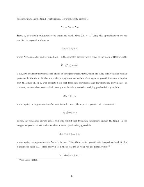
endogenous stochastic trend. Furthermore, log productivity growth is
∆zt = ∆at + ∆nt
Since, at is typically calibrated to be persistent shock, then ∆at ≈ ɛt. Using this approximation we can
rewrite the expression above as
∆zt = ∆nt + ɛt
where Also, since ∆nt is determined at t − 1, the expected growth rate is equal to the stock of R&D growth:
Et−1[∆zt] = ∆nt
Thus, low-frequency movements are driven by endogenous R&D rates, which are fairly persistent and volatile
processes in the data. Furthermore, the propagation mechanism of endogenous growth framework implies
that the single shock at will generate both high-frequency movements and low-frequency movements. In
contrast, in a standard neoclassical paradigm with a deterministic trend, log productivity growth is
∆zt = µ + ɛt
where again, the approximation ∆at ≈ ɛt is used. Hence, the expected growth rate is constant:
Et−1[∆zt] = µ
Hence, the exogenous growth model will only exhibit high-frequency movements around the trend. In the
exogenous growth model with a stochastic trend, productivity growth is
∆zt = µ + xt−1 + ɛt
where again, the approximation ∆at ≈ ɛt is used. Thus the expected growth rate is equal to the drift plus
a persistent shock xt−1, often referred to in the literature as “long-run productivity risk” 15
15 See Croce (2010).
Et−1[∆zt] = µ + xt−1
14