Precise Orbit Determination of Global Navigation Satellite System of ...

More documents

Recommendations

Info

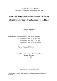
Chapter 5 Perturbation Models of IGSO,GEO and MEO Satellites Orbits Difference (meter) 3500 2500 1500 500 -500 -1500 -2500 -3500 dx dy dz 0 24 48 72 96 120 Tim e (hour) 144 168 192 216 240 5.4 Other Perturbations Figure 5-30 Effect of the Solar Radiation on Inclined Geostationary Satellite Other important perturbations such as ocean tide, solid earth tide, permanent tide, station displacement due to Pole tide and solid earth tide, ocean loading and so on have very small influences on IGSO and GEO satellites compared to the perturbations discussed above, but to MEO satellite (like GPS) some of these perturbations may be considered. 5.4.1 Solid Earth Tides Actually the earth can be considered as the elastic one, the attraction of the Sun and Moon on the earth will cause the earth mass to respond periodically by deforming and thus changing the earth’s geopotential and displacing the tracking station positions. This phenomenon is called solid earth tides. According to McCarthy (1992), solid earth tides are most easily modeled as variations in the standard geopotential coefficients Cnm and Snm , and can be calculated by two steps. First step uses a frequency independent Love number κ 2 (assuming κ 2 = 03 . ) and an evaluation of the tidal potential in the time domain from a lunar and solar ephemeris. The changes in normalized second degree geopotential coefficients for this step can be describes as follows 1 R GM j ∆C20 = κ 2 P 3 20 (sin φ j ) (5-42) 5 GM r 3 3 e � ⊕ j= 2 3 3 e � ⊕ j= 2 j 1 3 R GM j ∆C21 = κ 2 P 3 21(sinφ j ) cos λ j (5-43) 3 5 GM r 3 3 e � ⊕ j= 2 j 1 3 R GM j ∆S 21 = κ 2 P 3 21(sin φ j ) sin λ j (5-44) 3 5 GM r 3 3 e � ⊕ j= 2 j 1 12 R GM j ∆C22 = κ 2 P 3 22 (sin φ j ) cos λ j (5-45) 12 5 GM r 3 3 e � ⊕ j= 2 j 1 12 R GM j ∆S 22 = κ 2 P 3 22 (sin φ j ) sin λ j (5-46) 12 5 GM r where κ 2 Re GM ⊕ GM j j nominal second degree Love number equatorial radius of the Earth gravitational parameter for the Earth gravitational parameter for the Moon (j=2) and Sun (j=3) 62
Chapter 5 Perturbation Models of IGSO,GEO and MEO Satellites Orbits r j φ j λ j distance from geocenter to Moon or Sun body fixed geocentric latitude of Moon or Sun body fixed east longitude (from Greenwich) of Sun or Moon r j , φ j and λ j can be calculated by using JPL Planetary Ephemeris DE200. But Love number κ 2 is not constant according to Wahr model (Wahr, 1981) and dependent on the frequency. Thus the second step corrects the geopotential change computed in the first step by using the frequency dependent Love numbers. The changes in normalized coefficients from step 2 are � 1 � n + m ∆Cnm − i∆S nm = Am � δκ s H s � � � � �− i� n + m s( n, m) where even iθ s e odd (5-47) Am = R m ( −1) 4π ( 2 −δ , �1 δ om = � �0 m = 0 m ≠ 0 e om δks difference between Wahr model for κ at frequency s and the nominal value κ 2 in the sense κ s − κ 2 Hs amplitude (m) of term at frequency s from the Cartwright and Tayler (1971) and Cartwright and Edden (1973) harmonic expansion of the tide generating potential. The accelerations of IGSO and GEO satellite caused by solid earth tides are about 4.0×10 -10 m/s 2 ; the acceleration of MEO (GPS) satellite is about 3×10 -9 m/s 2 (Landau, 1988, Feltens 1991). From Table 5-1 to Table 5-4 we can conclude that the solid earth tides will cause the orbit errors of IGSO and GEO satellite about 0.10 m after one day arc; for MEO satellite the orbit error about 0.3 m (Landau, 1988), therefore this perturbation effect can be neglected from the satellite dynamical model for real-time orbit determination, because usually update step in orbit determination is short than 10 minutes and the influence from solid earth tides is very small; but for long period of orbit prediction or batch processing for post-processing, the solid earth tides should be included in the satellite dynamical models. The solid earth tides also displace the tracking station coordinates. According to Chadwell (1995, pp.30), the correction has a maximum at ϕ = 45 ο and is 0.013 m. Therefore this correction can also be neglected in the orbit determination of GNSS-2 satellites. 5.4.2 Ocean Tides Ocean tides are also caused by the attraction of the Sun and Moon on the Earth’s ocean that make the distribution of Earth’s mass changes periodically. The exact modeling of ocean tides of the earth is a difficult problem due to the complex hydrodynamic response to the tidal forces. Approximatly the same as the solid earth tides, the dynamical effect of ocean tides is most easily described as periodic variations in the normalized geopotential coefficients. The variations can be written as (Eanes, et al., 1983) ∆C nm − i∆S nm where 4πGρ Fnm = g w = F g = 9. 798261 ms -1 −11 �� − nm + s( n, m) ( C ± snm ± ( n + m)! ( n − m)! ( 2n + 1)( 2 −δ 3 −1 −2 iS om ± snm ) e ± iθ s 1+ κ n′ ) 2n + 1 G = 6. 673× 10 m kg s the gravitational constant ρ w κ ′ n = 1025kgm −3 ± C ± , S load deformation coefficients ( κ 2′ = −0. 3075, κ 3′ = −0. 195, κ 4′ = −0. 132, κ 5′ = −0. 1032, κ 6′ = −0. 0892 ) ocean tide coefficients in m for the tide constituent s snm snm The computation detail is referred to McCarthy (1992). 63 (5-48)
Page 1:
PRECISE ORBIT DETERMINATION OF GLOB
Page 4 and 5:
Summary GNSS-2 (Global Navigation S
Page 6 and 7:
3.2.2.1 Principle..................
Page 8 and 9:
9.3.3 The Effect of Distribution of
Page 10 and 11:
Chapter 1 Introduction 1.2 Developm
Page 12 and 13:
Chapter 2 Observations of Orbit Det
Page 14 and 15:
Page 16 and 17:
Page 18 and 19:
Page 20 and 21: Chapter 2 Observations of Orbit Det
Page 26 and 27: Chapter 3 Orbit Tracking System and
Page 40 and 41: Chapter 4 Major Error Sources of Sa
Page 52 and 53: Chapter 5 Perturbation Models of IG
Page 74 and 75: Chapter 6 Algorithms of Orbit Deter
Page 94 and 95: Chapter 7 Orbit Determination Using
Page 104 and 105: Chapter 8 Geostationary Orbit Deter
Page 120 and 121:
Chapter 8 Geostationary Orbit Deter
Page 122 and 123:
Chapter 9 Software and Simulation R
Page 124 and 125:
Page 126 and 127:
Page 128 and 129:
Page 130 and 131:
Page 132 and 133:
Page 134 and 135:
Page 136 and 137:
Page 138 and 139:
Page 140 and 141:
Page 142 and 143:
Page 144 and 145:
Page 146 and 147:
Page 148 and 149:
Page 150 and 151:
Page 152 and 153:
Conclusion 144
Page 154 and 155:
References Carpino M. (1995): SAEG
Page 156 and 157:
References Klobuchar, J. A.(1996):
Page 158 and 159:
References Traquilla, J. M. and J.
Page 160 and 161:
Acknowledgments 152
show all

Precise Orbit Determination of Global Navigation Satellite System of ...

You also want an ePaper? Increase the reach of your titles

Delete template?

Save as template?