Corynebacterium glutamicum - JUWEL - Forschungszentrum Jülich

2. Theory
evaluation can be made by comparing the achieved ˜χ 2 with values from standard chi
squared tables. The strict use of this rule might be difficult for dynamic fermentation
processes. Often, models are used with success although they probably do not meet the
chi squared rule. As also discussed in paragraph 2.2 on page 9, a severe simplification of
the complex system has to be made in order to get models which might be suitable for
process optimization and control. Furthermore it is often difficult to estimate the real
standard deviation of some of the measurements. The real measurement error of dilution
steps and the measurement equipment can usually easily be determined. Possible errors
by non-homogeneous samples, time delays in the off-line measurements et cetera, may
be more difficult to estimate. These errors can cause higher standard deviations and a
relatively high amount of outliers. Therefore, the choice of whether to reject a model is
usually not done solely based on a little bit too high a ˜χ 2 . Still the reduced chi squared
value forms a very valuable quantitative measure for the goodness of the fit and can also
be used to compare the fit of different models. The weighting by the degree of freedom
in the reduced form of the chi squared value provides some favouring of more simple
models with less parameters.
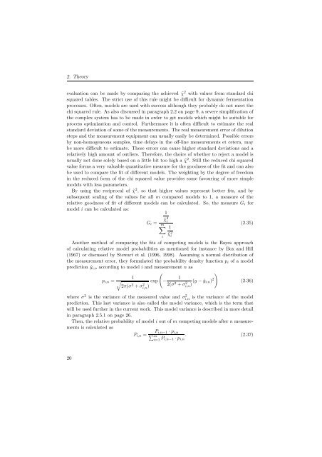
By using the reciprocal of ˜χ 2 , so that higher values represent better fits, and by
subsequent scaling of the values for all m compared models to 1, a measure of the
relative goodness of fit of different models can be calculated. So, the measure Gi for
model i can be calculated as:
Gi =
1
˜χ 2 i
m�
i
1
˜χ 2 i
(2.35)
Another method of comparing the fits of competing models is the Bayes approach
of calculating relative model probabilities as mentioned for instance by Box and Hill
(1967) or discussed by Stewart et al. (1996, 1998). Assuming a normal distribution of
the measurement error, they formulated the probability density function pi of a model
prediction ˆyi,n according to model i and measurement n as
�
�
pi,n =
1
�
2π(σ 2 + σ 2 i,n )
exp
−
1
2(σ2 + σ2 2
− ˆyi,n)
i,n )(y
(2.36)
where σ2 is the variance of the measured value and σ2 i,n is the variance of the model
prediction. This last variance is also called the model variance, which is the term that
will be used further in the current work. This model variance is described in more detail
in paragraph 2.5.1 on page 26.
Then, the relative probability of model i out of m competing models after n measurements
is calculated as
Pi,n−1 · pi,n
Pi,n = �m i=1 Pi,n−1
. (2.37)
· pi,n
20