transporte de solutos en el flujo de agua en riego por surcos - Helvia ...
transporte de solutos en el flujo de agua en riego por surcos - Helvia ...
transporte de solutos en el flujo de agua en riego por surcos - Helvia ...

You also want an ePaper? Increase the reach of your titles
YUMPU automatically turns print PDFs into web optimized ePapers that Google loves.
2. Mo<strong>de</strong>lo 1-D <strong>de</strong> <strong>flujo</strong> <strong>de</strong> <strong>agua</strong> y <strong>solutos</strong> <strong>en</strong> un surco <strong>de</strong> <strong>riego</strong><br />
22<br />
f<br />
Q<br />
− Q<br />
s<br />
= 0<br />
0 (2.12)<br />
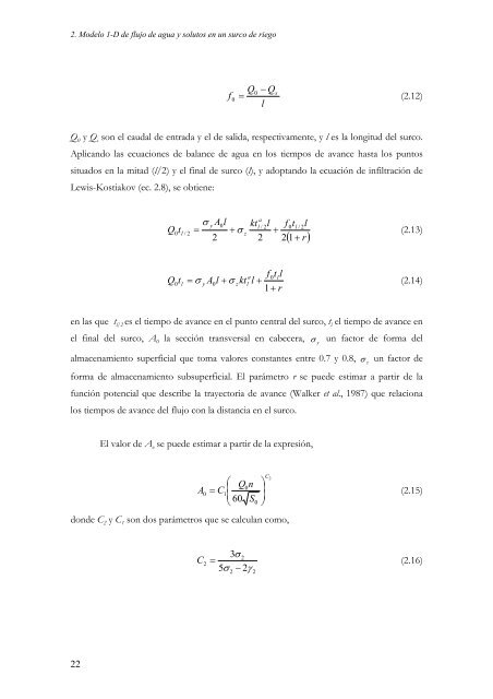
Q0 y Qs son <strong>el</strong> caudal <strong>de</strong> <strong>en</strong>trada y <strong>el</strong> <strong>de</strong> salida, respectivam<strong>en</strong>te, y l es la longitud <strong>de</strong>l surco.<br />
Aplicando las ecuaciones <strong>de</strong> balance <strong>de</strong> <strong>agua</strong> <strong>en</strong> los tiempos <strong>de</strong> avance hasta los puntos<br />
situados <strong>en</strong> la mitad (l/2) y <strong>el</strong> final <strong>de</strong> surco (l), y adoptando la ecuación <strong>de</strong> infiltración <strong>de</strong><br />
Lewis-Kostiakov (ec. 2.8), se obti<strong>en</strong>e:<br />
Q t<br />
0 l / 2<br />
Q t<br />
0 l<br />
a<br />
σ y A0l<br />
ktl<br />
/ 2l<br />
f t<br />
= + σ z +<br />
2 2 2<br />
l<br />
0 l / 2<br />
l<br />
( 1+<br />
r)<br />
(2.13)<br />
a f 0tl<br />
l<br />
= σ y A0l<br />
+ σ zktl<br />
l +<br />
(2.14)<br />
1+<br />
r<br />
<strong>en</strong> las que t l/2 es <strong>el</strong> tiempo <strong>de</strong> avance <strong>en</strong> <strong>el</strong> punto c<strong>en</strong>tral <strong>de</strong>l surco, t l <strong>el</strong> tiempo <strong>de</strong> avance <strong>en</strong><br />
<strong>el</strong> final <strong>de</strong>l surco, A0 la sección transversal <strong>en</strong> cabecera, σ un factor <strong>de</strong> forma <strong>de</strong>l<br />
y<br />
almac<strong>en</strong>ami<strong>en</strong>to superficial que toma valores constantes <strong>en</strong>tre 0.7 y 0.8, σ un factor <strong>de</strong><br />
z<br />
forma <strong>de</strong> almac<strong>en</strong>ami<strong>en</strong>to subsuperficial. El parámetro r se pue<strong>de</strong> estimar a partir <strong>de</strong> la<br />
función pot<strong>en</strong>cial que <strong>de</strong>scribe la trayectoria <strong>de</strong> avance (Walker et al., 1987) que r<strong>el</strong>aciona<br />
los tiempos <strong>de</strong> avance <strong>de</strong>l <strong>flujo</strong> con la distancia <strong>en</strong> <strong>el</strong> surco.<br />
El valor <strong>de</strong> A o se pue<strong>de</strong> estimar a partir <strong>de</strong> la expresión,<br />
A<br />
⎛<br />
⎜<br />
Q n ⎞<br />
⎟<br />
⎝ ⎠<br />
don<strong>de</strong> C2 y C1 son dos parámetros que se calculan como,<br />
C2<br />
0<br />
0 = C1<br />
(2.15)<br />
⎜ 60 S ⎟<br />
0<br />
3σ<br />
2 C 2 =<br />
(2.16)<br />
5σ<br />
2 − 2γ<br />
2