- Page 1 and 2:
Linear Algebra David Cherney, Tom D
- Page 3 and 4:
Contents 1 What is Linear Algebra?
- Page 5 and 6:
5 7.3 Properties of Matrices . . .
- Page 7 and 8:
7 16 Kernel, Range, Nullity, Rank 2
- Page 9 and 10:
What is Linear Algebra? 1 Many diff
- Page 11 and 12:
1.1 Organizing Information 11 ⎛
- Page 13 and 14:
1.2 What are Vectors? 13 (C) Polyno
- Page 15 and 16:
1.3 What are Linear Functions? 15 1
- Page 17 and 18:
1.3 What are Linear Functions? 17 W
- Page 19 and 20:
1.3 What are Linear Functions? 19 F
- Page 21 and 22:
1.4 So, What is a Matrix? 21 Each b
- Page 23 and 24:
1.4 So, What is a Matrix? 23 This i
- Page 25 and 26:
1.4 So, What is a Matrix? 25 We hav
- Page 27 and 28:
1.4 So, What is a Matrix? 27 = (2ax
- Page 29 and 30:
1.4 So, What is a Matrix? 29 Exampl
- Page 31 and 32:
1.5 Review Problems 31 Remember tha
- Page 33 and 34:
1.5 Review Problems 33 6. Matrix Mu
- Page 35 and 36:
1.5 Review Problems 35 (iv) Your an
- Page 37 and 38:
Systems of Linear Equations 2 2.1 G
- Page 39 and 40:
2.1 Gaussian Elimination 39 Entries
- Page 41 and 42:
2.1 Gaussian Elimination 41 called
- Page 43 and 44:
2.1 Gaussian Elimination 43 Algorit
- Page 45 and 46:
2.1 Gaussian Elimination 45 Advance
- Page 47 and 48:
2.1 Gaussian Elimination 47 ⎧ ⎪
- Page 49 and 50:
2.2 Review Problems 49 2. Solve the
- Page 51 and 52:
2.2 Review Problems 51 8. Show that
- Page 53 and 54:
2.3 Elementary Row Operations 53 Ex
- Page 55 and 56:
2.3 Elementary Row Operations 55 Ex
- Page 57 and 58:
2.3 Elementary Row Operations 57
- Page 59 and 60:
2.3 Elementary Row Operations 59 wh
- Page 61 and 62:
2.4 Review Problems 61 The LDU fact
- Page 63 and 64:
2.5 Solution Sets for Systems of Li
- Page 65 and 66:
2.5 Solution Sets for Systems of Li
- Page 67 and 68:
2.5 Solution Sets for Systems of Li
- Page 69 and 70:
2.6 Review Problems 69 so that a 2
- Page 71 and 72:
The Simplex Method 3 In Chapter 2,
- Page 73 and 74:
3.2 Graphical Solutions 73 3.2 Grap
- Page 75 and 76:
3.3 Dantzig’s Algorithm 75 Here w
- Page 77 and 78:
3.3 Dantzig’s Algorithm 77 ⎛
- Page 79 and 80:
3.4 Pablo Meets Dantzig 79 These ar
- Page 81 and 82:
3.5 Review Problems 81 their profit
- Page 83 and 84:
Vectors in Space, n-Vectors 4 To co
- Page 85 and 86:
4.2 Hyperplanes 85 4.2 Hyperplanes
- Page 87 and 88:
4.2 Hyperplanes 87 unless any of th
- Page 89 and 90:
4.3 Directions and Magnitudes 89 Th
- Page 91 and 92:
4.3 Directions and Magnitudes 91 Ex
- Page 93 and 94:
4.3 Directions and Magnitudes 93 Th
- Page 95 and 96:
4.4 Vectors, Lists and Functions: R
- Page 97 and 98:
4.5 Review Problems 97 4.5 Review P
- Page 99 and 100:
4.5 Review Problems 99 where the ve
- Page 101 and 102:
Vector Spaces 5 As suggested at the
- Page 103 and 104:
5.1 Examples of Vector Spaces 103 E
- Page 105 and 106:
5.1 Examples of Vector Spaces 105 E
- Page 107 and 108:
5.2 Other Fields 107 {( ∣∣∣ }
- Page 109 and 110:
5.3 Review Problems 109 5.3 Review
- Page 111 and 112:
Linear Transformations 6 The main o
- Page 113 and 114:
6.1 The Consequence of Linearity 11
- Page 115 and 116:
6.3 Linear Differential Operators 1
- Page 117 and 118:
6.4 Bases (Take 1) 117 sum of multi
- Page 119 and 120:
6.5 Review Problems 119 2. If f is
- Page 121 and 122:
Matrices 7 Matrices are a powerful
- Page 123 and 124:
7.1 Linear Transformations and Matr
- Page 125 and 126:
7.1 Linear Transformations and Matr
- Page 127 and 128:
7.1 Linear Transformations and Matr
- Page 129 and 130:
7.2 Review Problems 129 Linear oper
- Page 131 and 132:
7.2 Review Problems 131 (c) Find th
- Page 133 and 134:
7.3 Properties of Matrices 133 (m)
- Page 135 and 136:
7.3 Properties of Matrices 135 Exam
- Page 137 and 138:
7.3 Properties of Matrices 137 This
- Page 139 and 140:
7.3 Properties of Matrices 139 The
- Page 141 and 142:
7.3 Properties of Matrices 141 Some
- Page 143 and 144:
7.3 Properties of Matrices 143 •
- Page 145 and 146:
7.3 Properties of Matrices 145 7.3.
- Page 147 and 148:
7.4 Review Problems 147 ⎛ ⎞ ⎛
- Page 149 and 150:
7.4 Review Problems 149 Give a few
- Page 151 and 152:
7.5 Inverse Matrix 151 Figure 7.1:
- Page 153 and 154:
7.5 Inverse Matrix 153 At this poin
- Page 155 and 156:
7.6 Review Problems 155 Notice that
- Page 157 and 158:
7.6 Review Problems 157 (a) Compute
- Page 159 and 160:
7.7 LU Redux 159 7.7 LU Redux Certa
- Page 161 and 162:
7.7 LU Redux 161 ⎛ ⎞ u • Step
- Page 163 and 164:
7.7 LU Redux 163 so we would like t
- Page 165 and 166:
7.7 LU Redux 165 Reading homework:
- Page 167 and 168:
7.8 Review Problems 167 (k) Try to
- Page 169 and 170:
Determinants 8 Given a square matri
- Page 171 and 172:
8.1 The Determinant Formula 171 We
- Page 173 and 174:
8.1 The Determinant Formula 173 Thi
- Page 175 and 176:
8.2 Elementary Matrices and Determi
- Page 177 and 178:
8.2 Elementary Matrices and Determi
- Page 179 and 180:
8.2 Elementary Matrices and Determi
- Page 181 and 182:
8.2 Elementary Matrices and Determi
- Page 183 and 184: 8.3 Review Problems 183 Use row ope
- Page 185 and 186: 8.3 Review Problems 185 express you
- Page 187 and 188: 8.4 Properties of the Determinant 1
- Page 189 and 190: 8.4 Properties of the Determinant 1
- Page 191 and 192: 8.4 Properties of the Determinant 1
- Page 193 and 194: 8.5 Review Problems 193 Figure 8.8:
- Page 195 and 196: Subspaces and Spanning Sets 9 It is
- Page 197 and 198: 9.2 Building Subspaces 197 Note tha
- Page 199 and 200: 9.2 Building Subspaces 199 of the f
- Page 201 and 202: 9.2 Building Subspaces 201 Hence, t
- Page 203 and 204: 10 Linear Independence Consider a p
- Page 205 and 206: 10.1 Showing Linear Dependence 205
- Page 207 and 208: 10.2 Showing Linear Independence 20
- Page 209 and 210: 10.3 From Dependent Independent 209
- Page 211 and 212: 10.4 Review Problems 211 (b) If pos
- Page 213 and 214: 11 Basis and Dimension In chapter 1
- Page 215 and 216: 215 Worked Example Next, we would l
- Page 217 and 218: 11.1 Bases in R n . 217 a basis for
- Page 219 and 220: 11.2 Matrix of a Linear Transformat
- Page 221 and 222: 11.3 Review Problems 221 Alternativ
- Page 223 and 224: 11.3 Review Problems 223 6. Let S n
- Page 225 and 226: 12 Eigenvalues and Eigenvectors In
- Page 227 and 228: 12.1 Invariant Directions 227 as we
- Page 229 and 230: 12.1 Invariant Directions 229 Figur
- Page 231 and 232: 12.1 Invariant Directions 231 Readi
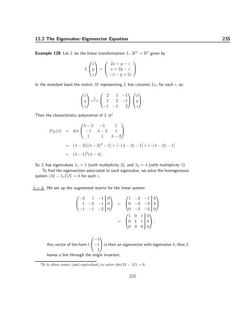
- Page 233: 12.2 The Eigenvalue-Eigenvector Equ
- Page 237 and 238: 12.3 Eigenspaces 237 is also an eig
- Page 239 and 240: 12.4 Review Problems 239 4. Let L b
- Page 241 and 242: 13 Diagonalization Given a linear t
- Page 243 and 244: 13.2 Change of Basis 243 Here, the
- Page 245 and 246: 13.2 Change of Basis 245 Meanwhile,
- Page 247 and 248: 13.3 Changing to a Basis of Eigenve
- Page 249 and 250: 13.4 Review Problems 249 (t n , . .
- Page 251 and 252: 13.4 Review Problems 251 (a) Show t
- Page 253 and 254: 14 Orthonormal Bases and Complement
- Page 255 and 256: 14.2 Orthogonal and Orthonormal Bas
- Page 257 and 258: 14.2 Orthogonal and Orthonormal Bas
- Page 259 and 260: 14.3 Relating Orthonormal Bases 259
- Page 261 and 262: 14.4 Gram-Schmidt & Orthogonal Comp
- Page 263 and 264: 14.4 Gram-Schmidt & Orthogonal Comp
- Page 265 and 266: 14.5 QR Decomposition 265 First, we
- Page 267 and 268: 14.6 Orthogonal Complements 267 vec
- Page 269 and 270: 14.6 Orthogonal Complements 269 The
- Page 271 and 272: 14.6 Orthogonal Complements 271 Exa
- Page 273 and 274: 14.7 Review Problems 273 (c) Suppos
- Page 275 and 276: 14.7 Review Problems 275 7. (a) Sho
- Page 277 and 278: 15 Diagonalizing Symmetric Matrices
- Page 279 and 280: 279 Example 141 The matrix M = ( )
- Page 281 and 282: 15.1 Review Problems 281 To diagona
- Page 283 and 284: 15.1 Review Problems 283 (b) Explai
- Page 285 and 286:
16 Kernel, Range, Nullity, Rank Giv
- Page 287 and 288:
16.2 Image 287 It might occur to yo
- Page 289 and 290:
16.2 Image 289 Figure 16.1: For the
- Page 291 and 292:
16.2 Image 291 Theorem 16.2.1. A fu
- Page 293 and 294:
16.2 Image 293 Example 148 of calcu
- Page 295 and 296:
16.2 Image 295 Thus ⎧⎛ ⎞ ⎛
- Page 297 and 298:
16.3 Summary 297 Reading homework:
- Page 299 and 300:
16.4 Review Problems 299 16.4 Revie
- Page 301 and 302:
16.4 Review Problems 301 Find the d
- Page 303 and 304:
17 Least squares and Singular Value
- Page 305 and 306:
305 However, the converse is often
- Page 307 and 308:
17.1 Projection Matrices 307 MX = V
- Page 309 and 310:
17.2 Singular Value Decomposition 3
- Page 311 and 312:
17.2 Singular Value Decomposition 3
- Page 313 and 314:
17.3 Review Problems 313 • v T M
- Page 315 and 316:
A List of Symbols ∈ ∼ R I n Pn
- Page 317 and 318:
B Fields Definition A field F is a
- Page 319 and 320:
Online Resources C Here are some in
- Page 321 and 322:
D Sample First Midterm Here are som
- Page 323 and 324:
323 8. What are the four main thing
- Page 325 and 326:
325 2. (a) The augmented matrix ⎛
- Page 327 and 328:
327 Since M T M −1 ≠ I, it foll
- Page 329 and 330:
329 (b) This is a vector space. Alt
- Page 331 and 332:
E Sample Second Midterm Here are so
- Page 333 and 334:
333 6. Suppose λ is an eigenvalue
- Page 335 and 336:
335 Thus ⎛ ⎞ ⎛ ⎞ ⎛ 3 1
- Page 337 and 338:
337 8. The associated eigenvalues s
- Page 339 and 340:
339 10. (i) We say that the vectors
- Page 341 and 342:
F Sample Final Exam Here are some w
- Page 343 and 344:
343 (h) Is M T M diagonalizable? (i
- Page 345 and 346:
345 after one orbit the satellite w
- Page 347 and 348:
347 (e) Is there a direction in whi
- Page 349 and 350:
349 well into the future. Then F 3
- Page 351 and 352:
351 Solutions (a) Write down a line
- Page 353 and 354:
353 Now solve UX = W by back substi
- Page 355 and 356:
355 Now zero out the top row by sub
- Page 357 and 358:
357 Finally, for λ = 3 2 ⎛ − 3
- Page 359 and 360:
359 11. (a) d2 X dt 2 (b) Since thi
- Page 361 and 362:
361 (b) Yes, the matrix M is symmet
- Page 363 and 364:
363 and since ker L = {0 V } we hav
- Page 365 and 366:
365 (b) The rows of M span (kerL)
- Page 367 and 368:
G Movie Scripts G.1 What is Linear
- Page 369 and 370:
G.2 Systems of Linear Equations 369
- Page 371 and 372:
G.2 Systems of Linear Equations 371
- Page 373 and 374:
G.2 Systems of Linear Equations 373
- Page 375 and 376:
G.2 Systems of Linear Equations 375
- Page 377 and 378:
G.3 Vectors in Space n-Vectors 377
- Page 379 and 380:
G.4 Vector Spaces 379 idea is to pl
- Page 381 and 382:
G.4 Vector Spaces 381 We are half-w
- Page 383 and 384:
G.5 Linear Transformations 383 You
- Page 385 and 386:
G.6 Matrices 385 G.6 Matrices Adjac
- Page 387 and 388:
G.6 Matrices 387 so this pair of ma
- Page 389 and 390:
G.6 Matrices 389 Hint for Review Qu
- Page 391 and 392:
G.6 Matrices 391 So this means that
- Page 393 and 394:
G.6 Matrices 393 Using an LU Decomp
- Page 395 and 396:
G.7 Determinants 395 we could fit t
- Page 397 and 398:
G.7 Determinants 397 2. As a matrix
- Page 399 and 400:
G.7 Determinants 399 ⎛ 1 Sj(λ) i
- Page 401 and 402:
G.7 Determinants 401 Now note that
- Page 403 and 404:
G.8 Subspaces and Spanning Sets 403
- Page 405 and 406:
G.9 Linear Independence 405 notion
- Page 407 and 408:
G.10 Basis and Dimension 407 G.10 B
- Page 409 and 410:
G.11 Eigenvalues and Eigenvectors 4
- Page 411 and 412:
G.11 Eigenvalues and Eigenvectors 4
- Page 413 and 414:
G.11 Eigenvalues and Eigenvectors 4
- Page 415 and 416:
G.12 Diagonalization 415 G.12 Diago
- Page 417 and 418:
G.12 Diagonalization 417 fruit (s,
- Page 419 and 420:
G.12 Diagonalization 419 Note that
- Page 421 and 422:
G.13 Orthonormal Bases and Compleme
- Page 423 and 424:
G.13 Orthonormal Bases and Compleme
- Page 425 and 426:
G.13 Orthonormal Bases and Compleme
- Page 427 and 428:
G.13 Orthonormal Bases and Compleme
- Page 429 and 430:
G.14 Diagonalizing Symmetric Matric
- Page 431 and 432:
G.15 Kernel, Range, Nullity, Rank 4
- Page 433 and 434:
Index Action, 389 Angle between vec
- Page 435 and 436:
INDEX 435 Linearly independent, 204