- Page 1:
UNIVERSITE DE LIMOGES ECOLE DOCTORA
- Page 5 and 6:
Sommaire SOMMAIRE INTRODUCTION GENE
- Page 7 and 8:
Sommaire III. Le résonateur ......
- Page 9:
INTRODUCTION GENERALE
- Page 12 and 13:
Introduction générale Parmi les f
- Page 15:
CHAPITRE I ANALYSE BIBLIOGRAPHIQUE
- Page 18 and 19:
Chapitre I : Analyse bibliographiqu
- Page 20 and 21:
Chapitre I : Analyse bibliographiqu
- Page 22 and 23:
Chapitre I : Analyse bibliographiqu
- Page 24 and 25:
Chapitre I : Analyse bibliographiqu
- Page 26 and 27:
Chapitre I : Analyse bibliographiqu
- Page 28 and 29:
Chapitre I : Analyse bibliographiqu
- Page 30 and 31:
Chapitre I : Analyse bibliographiqu
- Page 32 and 33:
Chapitre I : Analyse bibliographiqu
- Page 34 and 35:
Chapitre I : Analyse bibliographiqu
- Page 36 and 37:
Chapitre I : Analyse bibliographiqu
- Page 38 and 39:
Chapitre I : Analyse bibliographiqu
- Page 40 and 41:
Chapitre I : Analyse bibliographiqu
- Page 42 and 43:
Chapitre I : Analyse bibliographiqu
- Page 44 and 45:
Chapitre I : Analyse bibliographiqu
- Page 46 and 47:
Chapitre I : Analyse bibliographiqu
- Page 48 and 49:
Chapitre I : Analyse bibliographiqu
- Page 50 and 51:
Chapitre I : Analyse bibliographiqu
- Page 52 and 53:
Chapitre I : Analyse bibliographiqu
- Page 54 and 55:
Chapitre I : Analyse bibliographiqu
- Page 56 and 57:
Chapitre I : Analyse bibliographiqu
- Page 58 and 59:
Chapitre I : Analyse bibliographiqu
- Page 60 and 61:
Chapitre I : Analyse bibliographiqu
- Page 62 and 63:
Chapitre I : Analyse bibliographiqu
- Page 64 and 65:
Chapitre I : Analyse bibliographiqu
- Page 66 and 67:
Chapitre I : Analyse bibliographiqu
- Page 68 and 69:
Chapitre I : Analyse bibliographiqu
- Page 70 and 71:
Chapitre I : Analyse bibliographiqu
- Page 73 and 74:
Chapitre II : Inductance active I.
- Page 75 and 76:
Chapitre II : Inductance active uti
- Page 77 and 78:
Chapitre II : Inductance active gm2
- Page 79 and 80:
Chapitre II : Inductance active ) m
- Page 81 and 82:
Chapitre II : Inductance active A 2
- Page 83 and 84:
Chapitre II : Inductance active III
- Page 85 and 86:
Chapitre II : Inductance active B )
- Page 87 and 88: Chapitre II : Inductance active Cel
- Page 89 and 90: Chapitre II : Inductance active B )
- Page 91 and 92: Chapitre II : Inductance active III
- Page 93 and 94: Chapitre II : Inductance active N f
- Page 95 and 96: Chapitre II : Inductance active V.
- Page 97: CHAPITRE III AMPLIFICATEUR DIFFEREN
- Page 100 and 101: Chapitre III : Amplificateur diffé
- Page 102 and 103: Chapitre III : Amplificateur diffé
- Page 104 and 105: Chapitre III : Amplificateur diffé
- Page 106 and 107: Chapitre III : Amplificateur diffé
- Page 108 and 109: Chapitre III : Amplificateur diffé
- Page 110 and 111: Chapitre III : Amplificateur diffé
- Page 112 and 113: Chapitre III : Amplificateur diffé
- Page 114 and 115: Chapitre III : Amplificateur diffé
- Page 116 and 117: Chapitre III : Amplificateur diffé
- Page 118 and 119: Chapitre III : Amplificateur diffé
- Page 120 and 121: Chapitre III : Amplificateur diffé
- Page 122 and 123: Chapitre III : Amplificateur diffé
- Page 124 and 125: Chapitre III : Amplificateur diffé
- Page 126 and 127: Chapitre III : Amplificateur diffé
- Page 128 and 129: Chapitre III : Amplificateur diffé
- Page 131 and 132: Chapitre IV : Filtre actif LC compe
- Page 133 and 134: Chapitre IV : Filtre actif LC compe
- Page 135 and 136: Chapitre IV : Filtre actif LC compe
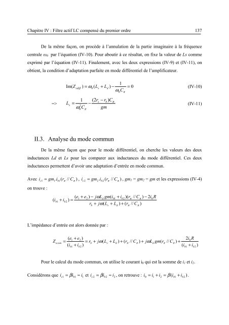
- Page 137: Chapitre IV : Filtre actif LC compe
- Page 141 and 142: Chapitre IV : Filtre actif LC compe
- Page 143 and 144: Chapitre IV : Filtre actif LC compe
- Page 145 and 146: Chapitre IV : Filtre actif LC compe
- Page 147 and 148: Chapitre IV : Filtre actif LC compe
- Page 149 and 150: Chapitre IV : Filtre actif LC compe
- Page 151 and 152: Chapitre IV : Filtre actif LC compe
- Page 153 and 154: Chapitre IV : Filtre actif LC compe
- Page 155 and 156: Chapitre IV : Filtre actif LC compe
- Page 157 and 158: Chapitre IV : Filtre actif LC compe
- Page 159 and 160: Chapitre IV : Filtre actif LC compe
- Page 161 and 162: Chapitre IV : Filtre actif LC compe
- Page 163 and 164: Chapitre IV : Filtre actif LC compe
- Page 165 and 166: Chapitre IV : Filtre actif LC compe
- Page 167 and 168: Chapitre IV : Filtre actif LC compe
- Page 169 and 170: Chapitre IV : Filtre actif LC compe
- Page 171 and 172: Chapitre IV : Filtre actif LC compe
- Page 173 and 174: Chapitre IV : Filtre actif LC compe
- Page 175 and 176: Chapitre IV : Filtre actif LC compe
- Page 177 and 178: Chapitre IV : Filtre actif LC compe
- Page 179 and 180: Chapitre IV : Filtre actif LC compe
- Page 181 and 182: Chapitre IV : Filtre actif LC compe
- Page 183 and 184: Chapitre IV : Filtre actif LC compe
- Page 185 and 186: Chapitre IV : Filtre actif LC compe
- Page 187 and 188: Chapitre IV : Filtre actif LC compe
- Page 189 and 190:
Chapitre IV : Filtre actif LC compe
- Page 191 and 192:
Chapitre IV : Filtre actif LC compe
- Page 193 and 194:
Chapitre IV : Filtre actif LC compe
- Page 195 and 196:
Chapitre IV : Filtre actif LC compe
- Page 197 and 198:
Chapitre IV : Filtre actif LC compe
- Page 199 and 200:
Chapitre IV : Filtre actif LC compe
- Page 201 and 202:
Chapitre IV : Filtre actif LC compe
- Page 203 and 204:
Chapitre IV : Filtre actif LC compe
- Page 205 and 206:
Chapitre IV : Filtre actif LC compe
- Page 207 and 208:
Chapitre IV : Filtre actif LC compe
- Page 209 and 210:
Chapitre IV : Filtre actif LC compe
- Page 211 and 212:
Chapitre IV : Filtre actif LC compe
- Page 213:
Chapitre IV : Filtre actif LC compe
- Page 217 and 218:
Perspective : Filtre passe-bande ut
- Page 219 and 220:
Perspective : Filtre passe-bande ut
- Page 221 and 222:
Perspective : Filtre passe-bande ut
- Page 223 and 224:
Perspective : Filtre passe-bande ut
- Page 225 and 226:
Perspective : Filtre passe-bande ut
- Page 227 and 228:
Perspective : Filtre passe-bande ut
- Page 229:
Perspective : Filtre passe-bande ut
- Page 233 and 234:
Conclusion générale Depuis longte
- Page 235:
ANNEXE I VALEUR DES ELEMENTS DU FIL
- Page 238 and 239:
Annexe I : Valeur des éléments du
- Page 240 and 241:
Annexe I : Valeur des éléments du
- Page 243 and 244:
Annexe II : Les paramètres S en mo
- Page 245 and 246:
Annexe II : Les paramètres S en mo
- Page 247 and 248:
Annexe II : Les paramètres S en mo
- Page 249:
ANNEXE III LES PROTECTIONS ANTENNES
- Page 252 and 253:
Annexe III : Les protections antenn
- Page 255 and 256:
Annexe IV : Modélisation des induc
- Page 257 and 258:
Annexe IV : Modélisation des induc
- Page 259:
ANNEXE V VALEUR DES ELEMENTS DE L
- Page 262 and 263:
Annexe V : Valeur des éléments de
- Page 264 and 265:
Annexe V : Valeur des éléments de
- Page 267:
ANNEXE VI SIMULATION ET MODELISATIO
- Page 270 and 271:
Annexe VI : Simulation et modélisa
- Page 272 and 273:
Annexe VI : Simulation et modélisa
- Page 274 and 275:
Annexe VI : Simulation et modélisa
- Page 276 and 277:
Annexe VI : Simulation et modélisa
- Page 278 and 279:
Annexe VI : Simulation et modélisa
- Page 280 and 281:
Annexe VI : Simulation et modélisa
- Page 283 and 284:
Annexe VII : Valeur des éléments
- Page 285 and 286:
Annexe VII : Valeur des éléments
- Page 287 and 288:
Annexe VII : Valeur des éléments
- Page 289:
ANNEXE VIII ARTICLES PERSONNELS
- Page 292 and 293:
Annexe IV : Articles personnels [6]
- Page 296:
Résumé Ces travaux de thèse cons