- Page 2 and 3:
FUNDAMENTAL SOLUTIONS IN ELASTODYNA
- Page 4 and 5:
Fundamental Solutions in Elastodyna
- Page 6 and 7: Contents Preface page ix SECTION I:
- Page 8 and 9: Contents vii SECTION V: ANALYTICAL
- Page 10 and 11: Preface We present in this work a c
- Page 12 and 13: SECTION I: PRELIMINARIES 1 Fundamen
- Page 14 and 15: 1.1 Notation and table of symbols 3
- Page 16 and 17: 1.3 Coordinate systems and differen
- Page 18 and 19: 1.3 Coordinate systems and differen
- Page 20 and 21: 1.3 Coordinate systems and differen
- Page 22 and 23: 1.3 Coordinate systems and differen
- Page 24 and 25: 1.4 Strains, stresses, and the elas
- Page 26 and 27: 1.4 Strains, stresses, and the elas
- Page 28 and 29: 1.4 Strains, stresses, and the elas
- Page 30 and 31: 1.4 Strains, stresses, and the elas
- Page 32 and 33: 1.4 Strains, stresses, and the elas
- Page 34 and 35: 1.4 Strains, stresses, and the elas
- Page 36 and 37: 1.4 Strains, stresses, and the elas
- Page 38 and 39: 2 Dipoles In most cases, we provide
- Page 40 and 41: 2.2 Line dipoles 29 z z z y y y x x
- Page 42 and 43: 2.5 Blast loads (explosive line and
- Page 44 and 45: 2.6 Dipoles in cylindrical coordina
- Page 46 and 47: SECTION II: FULL SPACE PROBLEMS 3 T
- Page 48 and 49: 3.3 SH line load in an orthotropic
- Page 50 and 51: 3.4 In-plane line load (SV-P waves)
- Page 52 and 53: 3.5 Dipoles in plane strain 41 0.6
- Page 54 and 55: 3.6 Line blast source: suddenly app
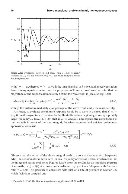
- Page 58 and 59: 3.7 Cylindrical cavity subjected to
- Page 60 and 61: 4.2 Point load (Stokes problem) 49
- Page 62 and 63: 4.2 Point load (Stokes problem) 51
- Page 64 and 65: 4.3 Tension cracks 53 given earlier
- Page 66 and 67: 4.5 Torsional point source 55 Spher
- Page 68 and 69: 4.6 Torsional point source with ver
- Page 70 and 71: 4.8 Spherical cavity subjected to a
- Page 72 and 73: 4.8 Spherical cavity subjected to a
- Page 74 and 75: 4.9 Spatially harmonic line source
- Page 76 and 77: 4.9 Spatially harmonic line source
- Page 78 and 79: 4.9 Spatially harmonic line source
- Page 80 and 81: SECTION III: HALF-SPACE PROBLEMS 5
- Page 82 and 83: 5.3 Half-plane, SV-P source and rec
- Page 84 and 85: 5.4 Half-plane, SV-P source on surf
- Page 86 and 87: 5.4 Half-plane, SV-P source on surf
- Page 88 and 89: 5.5 Half-plane, line blast load app
- Page 90 and 91: 6.1 3-D half-space, suddenly applie
- Page 92 and 93: 6.2 3-D half-space, suddenly applie
- Page 94 and 95: 6.3 3-D half-space, buried torsiona
- Page 96 and 97: 6.3 3-D half-space, buried torsiona
- Page 98 and 99: SECTION IV: PLATES AND STRATA 7 Two
- Page 100 and 101: 7.2 Stratum subjected to SH line so
- Page 102 and 103: 7.3 Plate with mixed boundary condi
- Page 104 and 105: 7.3 Plate with mixed boundary condi
- Page 106 and 107:
7.3 Plate with mixed boundary condi
- Page 108 and 109:
SECTION V: ANALYTICAL AND NUMERICAL
- Page 110 and 111:
8.1 Summary of results 99 Plane str
- Page 112 and 113:
8.2 Scalar Helmholtz equation in Ca
- Page 114 and 115:
8.3 Vector Helmholtz equation in Ca
- Page 116 and 117:
8.4 Elastic wave equation in Cartes
- Page 118 and 119:
8.4 Elastic wave equation in Cartes
- Page 120 and 121:
8.6 Vector Helmholtz equation in cy
- Page 122 and 123:
8.7 Elastic wave equation in cylind
- Page 124 and 125:
8.7 Elastic wave equation in cylind
- Page 126 and 127:
8.7 Elastic wave equation in cylind
- Page 128 and 129:
8.8 Scalar Helmholtz equation in sp
- Page 130 and 131:
8.9 Vector Helmholtz equation in sp
- Page 132 and 133:
8.10 Elastic wave equation in spher
- Page 134 and 135:
8.10 Elastic wave equation in spher
- Page 136 and 137:
9 Integral transform method The int
- Page 138 and 139:
9.1 Cartesian coordinates 127 In pa
- Page 140 and 141:
9.1 Cartesian coordinates 129 Writi
- Page 142 and 143:
9.2 Cylindrical coordinates 131 Fou
- Page 144 and 145:
9.2 Cylindrical coordinates 133 Hen
- Page 146 and 147:
9.2 Cylindrical coordinates 135 Oth
- Page 148 and 149:
9.3 Spherical coordinates 137 √
- Page 150 and 151:
9.3 Spherical coordinates 139 ∫
- Page 152 and 153:
10.1 Summary of method 141 special
- Page 154 and 155:
10.2 Stiffness matrix method in Car
- Page 156 and 157:
10.2 Stiffness matrix method in Car
- Page 158 and 159:
10.2 Stiffness matrix method in Car
- Page 160 and 161:
10.2 Stiffness matrix method in Car
- Page 162 and 163:
10.2 Stiffness matrix method in Car
- Page 164 and 165:
10.2 Stiffness matrix method in Car
- Page 166 and 167:
10.2 Stiffness matrix method in Car
- Page 168 and 169:
10.2 Stiffness matrix method in Car
- Page 170 and 171:
10.3 Stiffness matrix method in cyl
- Page 172 and 173:
10.3 Stiffness matrix method in cyl
- Page 174 and 175:
10.3 Stiffness matrix method in cyl
- Page 176 and 177:
10.3 Stiffness matrix method in cyl
- Page 178 and 179:
10.3 Stiffness matrix method in cyl
- Page 180 and 181:
10.3 Stiffness matrix method in cyl
- Page 182 and 183:
10.3 Stiffness matrix method in cyl
- Page 184 and 185:
10.3 Stiffness matrix method in cyl
- Page 186 and 187:
10.4 Stiffness matrix method for la
- Page 188 and 189:
10.4 Stiffness matrix method for la
- Page 190 and 191:
10.4 Stiffness matrix method for la
- Page 192 and 193:
10.4 Stiffness matrix method for la
- Page 194 and 195:
10.4 Stiffness matrix method for la
- Page 196 and 197:
SECTION VI: APPENDICES 11 Basic pro
- Page 198 and 199:
11.2 Spherical Bessel functions 187
- Page 200 and 201:
11.3 Legendre polynomials 189 1.0 P
- Page 202 and 203:
11.4 Associated Legendre functions
- Page 204 and 205:
11.4 Associated Legendre functions
- Page 206 and 207:
12.1 Fourier transforms 195 b) Wave
- Page 208 and 209:
12.3 Spherical Hankel transforms 19
- Page 210 and 211:
function [ ] = SH2D Full( ) 199 fun
- Page 212 and 213:
function [ ] = SVP2D Full(x, z, poi
- Page 214 and 215:
function [ ] = SVP2D Full(x, z, poi
- Page 216 and 217:
function [ ] = Blast2D(pois) 205 Ur
- Page 218 and 219:
function [ ] = Cavity2D(r, r0, pois
- Page 220 and 221:
function [ ] = Point Full(pois) 209
- Page 222 and 223:
function Torsion Full(x, y, z, td,
- Page 224 and 225:
function [ ] = Cavity3D(r, pois) 21
- Page 226 and 227:
function [ ] = SH2D Half(xs, zs, xr
- Page 228 and 229:
function [T, Ux, Uz] = Garvin(x, z,
- Page 230 and 231:
function [T, Uxx, Uxz, Uzz] = lamb2
- Page 232 and 233:
function [T, Uxx, Uxz, Uzz] = lamb2
- Page 234 and 235:
function [T, Uxx, Uxz, Uzz] = lamb2
- Page 236 and 237:
function [T, Uxx, Utx, Uzz, Urz] =
- Page 238 and 239:
function [T, Uxx, Utx, Uzz, Urz] =
- Page 240 and 241:
function [ ] = Torsion Half(r, z, z
- Page 242 and 243:
function [ ] = Torsion Half(r, z, z
- Page 244 and 245:
function [ ] = SH Plate(x, z, z0) 2
- Page 246 and 247:
function [ ] = SH Stratum(x, z, z0)
- Page 248 and 249:
function [ ] = SH Stratum(x, z, z0)
- Page 250 and 251:
function [ ] = SVP Plate(x, z, z0,
- Page 252 and 253:
function [ ] = SVP Plate(x, z, z0,
- Page 254 and 255:
function [ ] = SVP Plate(x, z, z0,
- Page 256 and 257:
function [ztors, zspher] = spheroid
- Page 258 and 259:
function [ztors, zspher] = spheroid
- Page 260 and 261:
function [si] = cisib(x) 249 functi
- Page 262:
function [el3] = ellipint3(phi, N,