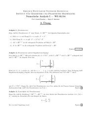
Aufgabe 1 Gegeben sei die Wertetabelle i 0 1 2 3 xi 0 1 2 4 fi â3 1 2 ...
Aufgabe 1 Gegeben sei die Wertetabelle i 0 1 2 3 xi 0 1 2 4 fi â3 1 2 ...
Aufgabe 1 Gegeben sei die Wertetabelle i 0 1 2 3 xi 0 1 2 4 fi â3 1 2 ...

Sie wollen auch ein ePaper? Erhöhen Sie die Reichweite Ihrer Titel.
YUMPU macht aus Druck-PDFs automatisch weboptimierte ePaper, die Google liebt.
Institut für Geometrie und Praktische Mathematik<br />
Höhere Mathematik IV (für Elektrotechniker und<br />
Technische Informatiker) - Numerik - SS 2007<br />
Dr. S. Börm , Dr. M. Larin<br />
Polynominterpolation<br />
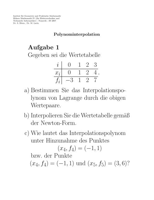
<strong>Aufgabe</strong> 1<br />
<strong>Gegeben</strong> <strong>sei</strong> <strong>die</strong> <strong>Wertetabelle</strong><br />
i 0 1 2 3<br />
x i 0 1 2 4<br />
f i −3 1 2 7<br />
a) Bestimmen Sie das Interpolationspolynom<br />
von Lagrange durch <strong>die</strong> obigen<br />
Wertepaare.<br />
b) Interpolieren Sie <strong>die</strong> <strong>Wertetabelle</strong> gemäß<br />
der Newton-Form.<br />
c) Wie lautet das Interpolationspolynom<br />
unter Hinzunahme des Punktes<br />
(x 4 , f 4 ) = (−1, 1)<br />
bzw. der Punkte<br />
(x 4 , f 4 ) = (−1, 1) und (x 5 , f 5 ) = (3, 6)?<br />
.
Polynominterpolation 2<br />
P 4 (x) =<br />
4∑<br />
f(x j ) l j4 (x)<br />
j=0<br />
= (−3) · x − 1<br />
0 − 1 · x − 2<br />
0 − 2 · x − 4<br />
0 − 4 · x + 1<br />
0 + 1<br />
+1 · x − 0<br />
1 − 0 · x − 2<br />
1 − 2 · x − 4<br />
1 − 4 · x + 1<br />
1 + 1<br />
+2 · x − 0<br />
2 − 0 · x − 1<br />
2 − 1 · x − 4<br />
2 − 4 · x + 1<br />
2 + 1<br />
+7 · x − 0<br />
4 − 0 · x − 1<br />
4 − 1 · x − 2<br />
4 − 2 · x + 1<br />
4 + 1<br />
x − 0<br />
+1 ·<br />
−1 − 0 · x − 1<br />
−1 − 1 · x − 2<br />
−1 − 2 ·<br />
= 7 15 x4 − 83<br />
30 x3 + 53<br />
15 x2 + 83<br />
30 x − 3.<br />
x − 4<br />
−1 − 4
Institut für Geometrie und Praktische Mathematik<br />
Höhere Mathematik IV (für Elektrotechniker und<br />
Technische Informatiker) - Numerik - SS 2007<br />
Dr. S. Börm , Dr. M. Larin<br />
Polynominterpolation: Lagrange-Form<br />
Die Lagrangschen Grundpolynome lauten<br />
n∏ x − x<br />
l jn (x) =<br />
k<br />
, j = 0, . . . , n.<br />
x i − x k<br />
k = 0<br />
k ≠ j<br />
Sie haben <strong>die</strong> Eigenschaft<br />
l jn (x i ) = δ ji , i, j = 0, . . . , n,<br />
wobei δ ji das Kronecker–Symbol bezeichnet.<br />
In der Lagrange-Darstellung lautet <strong>die</strong> Interpolationspolynom<br />
n∑<br />
P n (x) = f(x j )l jn (x).<br />
j=0
Institut für Geometrie und Praktische Mathematik<br />
Höhere Mathematik IV (für Elektrotechniker und<br />
Technische Informatiker) - Numerik - SS 2007<br />
Dr. S. Börm , Dr. M. Larin<br />
Polynominterpolation: Newton-Form<br />
Die Newton-Basis lautet<br />
w 0 (x) = 1, w k (x) =<br />
k−1<br />
∏<br />
(x − x i ),<br />
i=0<br />
mit k = 0, . . . , n. Die divi<strong>die</strong>rten Differenzen<br />
berechnen sich rekursiv nach der Formel<br />
[x 0 , . . . , x n ]f = [x 1,...,x n ]f−[x 0 ,...,x n−1 ]f<br />
x n −x 0<br />
mit [x i ]f = f(x i ). Das Interpolationspolynom<br />
in der Newton–Form lautet<br />
n∑<br />
P n (x) = [x 1 , . . . , x k+1 ]f · w k (x).<br />
k=0
Institut für Geometrie und Praktische Mathematik<br />
Höhere Mathematik IV (für Elektrotechniker und<br />
Technische Informatiker) - Numerik - SS 2007<br />
Dr. S. Börm , Dr. M. Larin<br />
Polynominterpolation<br />
<strong>Aufgabe</strong> 2<br />
Sei f(x) = e x und p(x) ∈ P 3 dasjenige<br />
Polynom, das f(x) an den Stellen<br />
x 0 = −1, x 1 = 0, x 2 = 1, x 3 = 2,<br />
interpoliert.<br />
a) Geben Sie p(x) in der Newton-Form<br />
an.<br />
b) Wie groß kann der Interpolationfehler<br />
im Interval [1, 2] höchstens werden?<br />
c) Wie läßt er sich an der Stelle x = 1 2<br />
abschätzen und wie groß ist er tatsächlich?
Institut für Geometrie und Praktische Mathematik<br />
Höhere Mathematik IV (für Elektrotechniker und<br />
Technische Informatiker) - Numerik - SS 2007<br />
Dr. S. Börm , Dr. M. Larin<br />
Polynominterpolation: Fehlerabschätzung<br />
Für x i ∈ [a, b] und f ∈ R n+1 [a, b] gilt<br />
f(x) − P n (x) = f (n+1) (ξ)<br />
(n + 1)!<br />
wobei ξ ∈ [a, b] und<br />
· ω n+1 (x),<br />
ω n+1 (x) = (x − x 0 )(x − x 1 ) . . . (x − x n ).<br />
Die Fehlerabschätzung auf [a, b]:<br />
f (n+1) (ξ)<br />
|f(x) − p n (x)| =<br />
· ω<br />
∣ (n + 1)! n+1 (x)<br />
∣<br />
f (n+1) (x)<br />
≤ max<br />
x∈[a,b] ∣ (n + 1)! ∣ · max |ω n+1(x)|<br />
x∈[a,b]
Institut für Geometrie und Praktische Mathematik<br />
Höhere Mathematik IV (für Elektrotechniker und<br />
Technische Informatiker) - Numerik - SS 2007<br />
Dr. S. Börm , Dr. M. Larin<br />
<strong>Aufgabe</strong> 3<br />
Die Funktion<br />
Polynominterpolation<br />
f(x) := 2 sin(3πx)<br />
soll durch Polynome an den Stützstellen<br />
interpoliert werden.<br />
x 1 = 0, x 2 = 1 12 , x 3 = 1 6 , x 4 = 1 3<br />
a) Werten Sie das Interpolationspolynom P (f|x 1 , x 2 , x 4 )(x)<br />
an der Stelle x = 1 10<br />
mit dem Aitken-Neville-Schema<br />
aus.<br />
b) Bestimmen Sie <strong>die</strong> Lagrange- und <strong>die</strong> Newton-Darstellung<br />
des Polynoms P (f|x 1 , x 2 , x 3 )(x).<br />
c) Werten Sie <strong>die</strong> Newton-Darstellung aus Teilaufgabe b)<br />
mit dem Horner-Schema an den Stellen y 1 = 1 10 und<br />
y 2 = 1 8 aus.<br />
d) Schätzen Sie den Interpolationsfehler |P (f|x 1 , x 2 , x 3 )(x) − f(x)|<br />
im Intervall [0, 1 6 ] ab.<br />
e) Ermitteln Sie das Interpolationspolynom P (f|x 1 , x 2 , x 3 , x 4 )(x).<br />
Welche Darstellung wählen Sie?
Institut für Geometrie und Praktische Mathematik<br />
Höhere Mathematik IV (für Elektrotechniker und<br />
Technische Informatiker) - Numerik - SS 2007<br />
Dr. S. Börm , Dr. M. Larin<br />
Polynominterpolation: Horner-Schema<br />
Zur Berechnung des Wertes des Polynom<br />
n∑<br />
P n (a) = c k w k (a) = c 0 + (a − x 0 )(c 1<br />
k=0<br />
+ . . . (c n−1 + (a − x n−1 )c n ) . . .)).<br />
mit c k = [x 1 , . . . , x k+1 ]f an der Stelle x = a<br />
benutzt man eine ef<strong>fi</strong>ziente Methode<br />
Setze p := c n .<br />
Für k = n − 1, . . . , 0 berechne<br />
s = c k + (a − x k )p
Institut für Geometrie und Praktische Mathematik<br />
Höhere Mathematik IV (für Elektrotechniker und<br />
Technische Informatiker) - Numerik - SS 2007<br />
Dr. S. Börm , Dr. M. Larin<br />
Polynominterpolation: Neville-Aitken-Schema<br />
Lemma 8.6.<br />
P i,k = x−x i−k<br />
x i −x i−k<br />
P i,k−1 +<br />
x i−x<br />
x i −x i−k<br />
P i−1,k−1<br />
= P i,k−1 + u i−u<br />
u i −u i−k<br />
(P i−1,k−1 − P i,k−1 )<br />
für 0 ≤ k ≤ i ≤ n.
Institut für Geometrie und Praktische Mathematik<br />
Höhere Mathematik IV (für Elektrotechniker und<br />
Technische Informatiker) - Numerik - SS 2007<br />
Dr. S. Börm , Dr. M. Larin<br />
<strong>Aufgabe</strong> 4<br />
Die Funktion<br />
Polynominterpolation<br />
f(x) =<br />
∫ x<br />
0<br />
sin 2 (t) dt<br />
soll im Intervall I = [0, π 2 ] äquidistant<br />
so tabelliert werden, daß bei linearer Interpolation<br />
der Interpolationsfehler für<br />
jedes x ∈ I kleiner als 0.25 · 10 −4 ist.<br />
Wie groß darf der Stützstellenabstand h<br />
dann höchstens <strong>sei</strong>n und wieviele Funktionswerte<br />
müssen in <strong>die</strong> Tabelle aufgenommen<br />
werden?
Institut für Geometrie und Praktische Mathematik<br />
Höhere Mathematik IV (für Elektrotechniker und<br />
Technische Informatiker) - Numerik - SS 2007<br />
Dr. S. Börm , Dr. M. Larin<br />
Polynominterpolation<br />
<strong>Aufgabe</strong> 5<br />
□ <strong>Gegeben</strong> <strong>sei</strong>en <strong>die</strong> reellen Stützstellen<br />
x 0 , x 1 , . . . , x n ∈ R mit<br />
x 0 < x 1 < · · · < x n<br />
und eine stetige Funktion f : R → R.<br />
Das Interpolationspolynom P (f|x 0 , . . . , x n )<br />
ist eindeutig bestimmt.<br />
□ <strong>Gegeben</strong> <strong>sei</strong>en <strong>die</strong> reellen Stützstellen<br />
x 0 , x 1 , . . . , x n ∈ R mit<br />
x 0 < x 1 < · · · < x n<br />
und eine stetige Funktion f : R → R.<br />
Sei τ ∈ S {0,1,...,n} eine Permutation<br />
der Punkte 0 bis n. Dann gilt<br />
P (f|x 0 , x 1 , . . . , x n ) =<br />
P (f|x τ(0) , x τ(1) , . . . , x τ(n) ).
Institut für Geometrie und Praktische Mathematik<br />
Höhere Mathematik IV (für Elektrotechniker und<br />
Technische Informatiker) - Numerik - SS 2007<br />
Dr. S. Börm , Dr. M. Larin<br />
<strong>Aufgabe</strong> 5<br />
Polynominterpolation<br />
□ Seien [a, b] ⊂ R ein kompaktes Intervall<br />
und f : [a, b] → R (n + 1)-mal<br />
stetig differenzierbar. Dann läßt sich<br />
der Appro<strong>xi</strong>mationsfehler abschätzen<br />
durch<br />
max |f−P n| ≤ max |ω n|· max<br />
x∈[a,b] x∈[a,b] x∈[a,b]<br />
|f (n) (x)|<br />
(n + 1)! .<br />
□ Es <strong>sei</strong> l i,n (x) <strong>die</strong> Lagrange–Grundpolynome<br />
zu den Stützstellen x 0 , . . . , x n , n ≥ 1,<br />
dann gilt<br />
n∑<br />
(x + 1) n = l i,n (x)(x i + 1)<br />
i=0<br />
für alle x ∈ [x 0 , x n ].