Xcell Journal Issue 78: Charge to Market with Xilinx 7 Series ...

XPLANATION: FPGA 101
FIR filter implementation using both classical DSP and
FPGA architectures to illustrate some of the strengths and
weaknesses of each solution.
EXAMPLE: A DIGITAL FIR FILTER
One of the most widely used digital signal-processing elements
is the finite impulse response, or FIR, filter.
Designers use filters to alter the magnitude or frequency
content of a data signal, usually to isolate or accentuate a
particular region of interest within the sample data spectrum.
In this regard, you can think of filters as a method of
preconditioning a signal. In a typical filter application,
incoming data samples combine with filter coefficients
through carefully synchronized mathematical operations,
which are dependent on the filter type and implementation
strategy, and then move on to the next processing stage. If
the data source and destination are analog signals, then
the samples must first pass through an A/D converter, and
the results fed through a D/A converter.
The simplest form of a FIR filter is implemented
through a series of delay elements, multipliers and an
adder tree or chain.
Mathematically, this equation describes the single-channel
FIR filter:
You can think of the terms in the equation as input samples,
output samples and coefficients. If S is a continuous
stream of input samples and Y is the resulting filtered
stream of output samples, then n and k correspond to a particular
instant in time. Thus, to compute the output sample
Y(n) at time n, a group of samples at N different points in
time, or s(n), s(n-1), s(n-2), … s(n-N+1), is required. The
group of N input samples is multiplied by N coefficients
and summed together to form the final result, Y.
Coefficient
Delay
S(n)
12
k 0 k 1 k 1 k 3 k 30
Multiply
Z -1 Z -1 Z -1 Z -1
Σ
y(n)
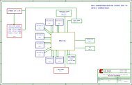
Figure 2 – FIR filter of length 31
Summation
Figure 2 is a block diagram for a simple 31-tap FIR filter
(length N = 31).
Various design tools are available to help select the ideal
length of a filter and the coefficient values. The goal is to
select the appropriate parameters to achieve the required
filter performance. The most popular design tool for choosing
these parameters is MATLAB ® . Once you have selected
the filter parameters, the implementation follows the mathematical
equation.
The basic steps for implementation of an FIR filter are:
1. Sample the incoming data stream.
2. Organize the input samples in a buffer so that each captured
sample may be multiplied by each filter coefficient.
3. Multiply each data sample by each coefficient and
accumulate the result.
4. Output filtered result.
A typical C program for implementing this FIR filter on a
processor using a multiply–accumulate approach is shown
in the code below.
/*
* Capture the incoming data samples
*/
datasample = input();
/*
* Push the new data sample onto the buffer
*/
S[n] = datasample;
/*
* Multiply each data sample by each coefficient
and accumulate the result
*/
y = 0;
for (i = 0; i