SAS/STAT 9.2 User's Guide: The MIXED Procedure (Book Excerpt)

More documents

Recommendations

Info

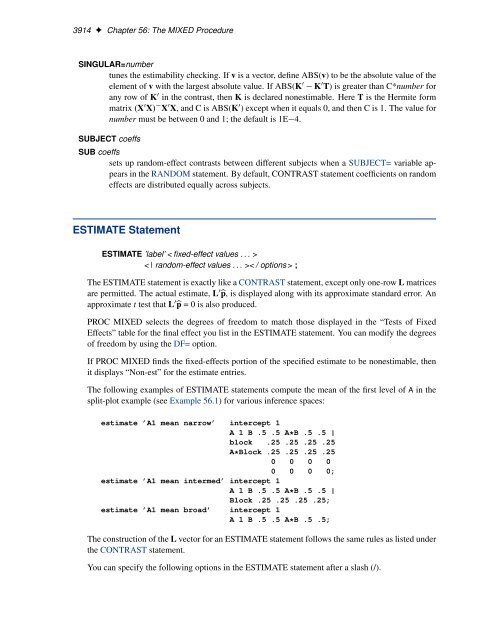
3914 ✦ Chapter 56: The MIXED Procedure SINGULAR=number tunes the estimability checking. If v is a vector, define ABS(v) to be the absolute value of the element of v with the largest absolute value. If ABS(K 0 K 0 T) is greater than C*number for any row of K 0 in the contrast, then K is declared nonestimable. Here T is the Hermite form matrix .X 0 X/ X 0 X, and C is ABS(K 0 ) except when it equals 0, and then C is 1. The value for number must be between 0 and 1; the default is 1E 4. SUBJECT coeffs SUB coeffs sets up random-effect contrasts between different subjects when a SUBJECT= variable appears in the RANDOM statement. By default, CONTRAST statement coefficients on random effects are distributed equally across subjects. ESTIMATE Statement ESTIMATE ’label’ < fixed-effect values . . . > < | random-effect values . . . >< / options > ; The ESTIMATE statement is exactly like a CONTRAST statement, except only one-row L matrices are permitted. The actual estimate, L 0 bp, is displayed along with its approximate standard error. An approximate t test that L 0 bp = 0 is also produced. PROC MIXED selects the degrees of freedom to match those displayed in the “Tests of Fixed Effects” table for the final effect you list in the ESTIMATE statement. You can modify the degrees of freedom by using the DF= option. If PROC MIXED finds the fixed-effects portion of the specified estimate to be nonestimable, then it displays “Non-est” for the estimate entries. The following examples of ESTIMATE statements compute the mean of the first level of A in the split-plot example (see Example 56.1) for various inference spaces: estimate ’A1 mean narrow’ intercept 1 A 1 B .5 .5 A*B .5 .5 | block .25 .25 .25 .25 A*Block .25 .25 .25 .25 0 0 0 0 0 0 0 0; estimate ’A1 mean intermed’ intercept 1 A 1 B .5 .5 A*B .5 .5 | Block .25 .25 .25 .25; estimate ’A1 mean broad’ intercept 1 A 1 B .5 .5 A*B .5 .5; The construction of the L vector for an ESTIMATE statement follows the same rules as listed under the CONTRAST statement. You can specify the following options in the ESTIMATE statement after a slash (/).
ESTIMATE Statement ✦ 3915 ALPHA=number requests that a t-type confidence interval be constructed with confidence level 1 number. The value of number must be between 0 and 1; the default is 0.05. CL requests that t-type confidence limits be constructed. The confidence level is 0.95 by default; this can be changed with the ALPHA= option. DF=number specifies the degrees of freedom for the t test and confidence limits. The default is the denominator degrees of freedom taken from the “Tests of Fixed Effects” table and corresponds to the final effect you list in the ESTIMATE statement. DIVISOR=number specifies a value by which to divide all coefficients so that fractional coefficients can be entered as integer numerators. E GROUP coeffs requests that the L matrix coefficients be displayed. For ODS purposes, the name of this “L Matrix Coefficients” table is “Coef.” GRP coeffs sets up random-effect contrasts between different groups when a GROUP= variable appears in the RANDOM statement. By default, ESTIMATE statement coefficients on random effects are distributed equally across groups. LOWER LOWERTAILED requests that the p-value for the t test be based only on values less than the t statistic. A two-tailed test is the default. A lower-tailed confidence limit is also produced if you specify the CL option. SINGULAR=number tunes the estimability checking as documented for the SINGULAR= option in the CONTRAST statement. SUBJECT coeffs SUB coeffs sets up random-effect contrasts between different subjects when a SUBJECT= variable appears in the RANDOM statement. By default, ESTIMATE statement coefficients on random effects are distributed equally across subjects. For example, the ESTIMATE statement in the following code from Example 56.5 constructs the difference between the random slopes of the first two batches. proc mixed data=rc; class batch; model y = month / s; random int month / type=un sub=batch s; estimate ’slope b1 - slope b2’ | month 1 / subject 1 -1; run;
Page 1 and 2: SAS/STAT ® 9.2 User’s Guide The
Page 3 and 4: Chapter 56 The MIXED Procedure Cont
Page 5 and 6: Basic Features ✦ 3887 clustered i
Page 7 and 8: variance components compound symmet
Page 9 and 10: Clustered Data Example ✦ 3891 The
Page 11 and 12: Clustered Data Example ✦ 3893 mat
Page 13 and 14: criterion of 1E 8. Figure 56.11 REM
Page 15 and 16: Syntax: MIXED Procedure ✦ 3897 Th
Page 17 and 18: Table 56.2 continued Option Descrip
Page 19 and 20: If H k is singular, then PROC MIXED
Page 21 and 22: MMEQ PROC MIXED Statement ✦ 3903
Page 23 and 24: PLOTS < (global-plot-options ) > <
Page 25 and 26: Residual Plot Options PROC MIXED St
Page 27 and 28: RATIO Multiple Plot Request PROC MI
Page 29 and 30: CONTRAST Statement ✦ 3911 TRUNCAT
Page 31: CONTRAST Statement ✦ 3913 differe
Page 35 and 36: Table 56.5 Summary of Important LSM
Page 37 and 38: LSMEANS Statement ✦ 3919 The numb
Page 39 and 40: E LSMEANS Statement ✦ 3921 are di
Page 41 and 42: Table 56.6 continued Option Descrip
Page 43 and 44: Table 56.7 Aliases for DDFM= Option
Page 45 and 46: E E1 E2 E3 FULLX MODEL Statement
Page 47 and 48: MODEL Statement ✦ 3929 The modifi
Page 49 and 50: SIZE=n MODEL Statement ✦ 3931 ins
Page 51 and 52: Table 56.10 continued Suboption Sta
Page 53 and 54: MODEL Statement ✦ 3935 where Vm i
Page 55 and 56: PARMS Statement PARMS (value-list)
Page 57 and 58: OLS PRIOR Statement ✦ 3939 approp
Page 59 and 60: PRIOR Statement ✦ 3941 JEFFREYS s
Page 61 and 62: RANDOM Statement ✦ 3943 TDATA= en
Page 63 and 64: RANDOM Statement ✦ 3945 GCORR dis
Page 65 and 66: RANDOM Statement ✦ 3947 available
Page 67 and 68: Table 56.12 continued Option Descri
Page 69 and 70: proc mixed; class a; model y = a x;
Page 71 and 72: REPEATED Statement ✦ 3953 TYPE=co
Page 73 and 74: Table 56.15 Covariance Structure Ex
Page 75 and 76: REPEATED Statement ✦ 3957 TYPE=AR
Page 77 and 78: TYPE=SP(EXPGA)(c1 c2) TYPE=SP(GAUGA
Page 79 and 80: TYPE=UN@AR(1) TYPE=UN@CS REPEATED S
Page 81 and 82: Mixed Models Theory ✦ 3963 where
Page 83 and 84:
proc mixed; class indiv; model y =
Page 85 and 86:
2 6 Z D 6 4 2 6 G D 6 4 1 1 1 1 1 1
Page 87 and 88:
Mixed Models Theory ✦ 3969 In man
Page 89 and 90:
Mixed Models Theory ✦ 3971 Finall
Page 91 and 92:
Mixed Models Theory ✦ 3973 When L
Page 93 and 94:
Parameterization of Mixed Models
Page 95 and 96:
Interaction Effects Parameterizatio
Page 97 and 98:
Table 56.20 Example of Continuous-b
Page 99 and 100:
as ei ei p D pvi VarŒei and studen
Page 101 and 102:
Residuals and Influence Diagnostics
Page 103 and 104:
Page 105 and 106:
Page 107 and 108:
Default Output Default Output ✦ 3
Page 109 and 110:
Default Output ✦ 3991 batch proce
Page 111 and 112:
ODS Table Names ✦ 3993 You can us
Page 113 and 114:
Table 56.22 continued ODS Table Nam
Page 115 and 116:
Table 56.23 continued Table Name Va
Page 117 and 118:
ODS Graphics ✦ 3999 The graphical
Page 119 and 120:
ODS Graphics ✦ 4001 precision is
Page 121 and 122:
Table 56.24 continued ODS Graph Nam
Page 123 and 124:
Computational Issues ✦ 4005 For f
Page 125 and 126:
Memory Computational Issues ✦ 400
Page 127 and 128:
The following statements fit the sp
Page 129 and 130:
Output 56.1.6 Split-Plot Analysis (
Page 131 and 132:
proc mixed; class A B Block; model
Page 133 and 134:
Example 56.2: Repeated Measures ✦
Page 135 and 136:
Output 56.2.6 Repeated Measures Ana
Page 137 and 138:
Output 56.2.9 Repeated Measures Ana
Page 139 and 140:
Output 56.2.11 continued Dimensions
Page 141 and 142:
Output 56.2.17 Analysis with Compou
Page 143 and 144:
Example 56.2: Repeated Measures ✦
Page 145 and 146:
The results from this analysis are
Page 147 and 148:
Output 56.3.6 Estimated Covariance
Page 149 and 150:
Output 56.3.10 Solutions of the Mix
Page 151 and 152:
Output 56.3.14 Plot of Likelihood S
Page 153 and 154:
Example 56.4: Known G and R ✦ 403
Page 155 and 156:
Example 56.4: Known G and R ✦ 403
Page 157 and 158:
Output 56.4.9 Solutions of the Mixe
Page 159 and 160:
Example 56.5: Random Coefficients E
Page 161 and 162:
Output 56.5.3 continued Number of O
Page 163 and 164:
Output 56.5.9 Random Coefficients A
Page 165 and 166:
Example 56.5: Random Coefficients
Page 167 and 168:
Example 56.6: Line-Source Sprinkler
Page 169 and 170:
Output 56.6.3 Model Dimensions and
Page 171 and 172:
Example 56.6: Line-Source Sprinkler
Page 173 and 174:
Example 56.7: Influence in Heteroge
Page 175 and 176:
Example 56.7: Influence in Heteroge
Page 177 and 178:
Output 56.7.5 Covariance Parameter
Page 179 and 180:
Output 56.7.7 Restricted Likelihood
Page 181 and 182:
Output 56.7.9 Covariance Parameter
Page 183 and 184:
Example 56.8: Influence Analysis fo
Page 185 and 186:
Output 56.8.2 Restricted Likelihood
Page 187 and 188:
Page 189 and 190:
Page 191 and 192:
Output 56.8.8 Distribution of Condi
Page 193 and 194:
Output 56.9.2 Type 3 Tests in Split
Page 195 and 196:
Output 56.9.5 Parameter Estimates i
Page 197 and 198:
References ✦ 4079 Carroll, R. J.
Page 199 and 200:
References ✦ 4081 Hanks, R.J., Si
Page 201 and 202:
References ✦ 4083 Littell, R. C.,
Page 203 and 204:
References ✦ 4085 Smith, A. F. M.
Page 205 and 206:
Subject Index 2D geometric anisotro
Page 207 and 208:
graphics, residual panel, 3998 grap
Page 209 and 210:
maximum likelihood estimation mixed
Page 211 and 212:
parameterization, 3975 Pearson resi
Page 213:
subject effect MIXED procedure, 391
Page 216 and 217:
INFLUENCE option, MODEL statement (
Page 218 and 219:
OUTG= option, 3942 OUTGT= option, 3
Page 220 and 221:
INFLUENCE option, MODEL statement (
Page 223:
SAS® Publishing Delivers! Whether
show all

SAS/STAT 9.2 User's Guide: The MIXED Procedure (Book Excerpt)

Create successful ePaper yourself

Delete template?

Save as template?