- Page 1 and 2:
Numerical Methods for the Wigner-Po
- Page 3 and 4:
NUMERICAL METHODS FOR THE WIGNER-PO
- Page 5 and 6:
Acknowledgments First and foremost,
- Page 7 and 8:
Table of Contents List of Tables ix
- Page 9 and 10:
4.3 ApplicationofSchauder’sFixedP
- Page 11 and 12:
List of Tables 1.1 PhysicalConstant
- Page 13 and 14:
3.11 I-V Curve with 30 Percent Redu
- Page 15 and 16:
CHAPTER 1. OVERVIEW 2 being heavily
- Page 17 and 18:
CHAPTER 1. OVERVIEW 4 Doping Spacer
- Page 19 and 20:
CHAPTER 1. OVERVIEW 6 and identfyin
- Page 21 and 22:
CHAPTER 1. OVERVIEW 8 for predictin
- Page 23 and 24:
CHAPTER 1. OVERVIEW 10 by Schrödin
- Page 25 and 26:
CHAPTER 1. OVERVIEW 12 ranging term
- Page 27 and 28:
CHAPTER 1. OVERVIEW 14 But because
- Page 29 and 30:
CHAPTER 1. OVERVIEW 16 = h 2π ,we
- Page 31 and 32:
CHAPTER 1. OVERVIEW 18 Table 1.1: P
- Page 33 and 34:
CHAPTER 1. OVERVIEW 20 where q is t
- Page 35 and 36:
CHAPTER 1. OVERVIEW 22 get K(f)
- Page 37 and 38:
CHAPTER 1. OVERVIEW 24 rule. The pr
- Page 39 and 40:
CHAPTER 1. OVERVIEW 26 The weights
- Page 41 and 42:
Chapter 2 Temporal Integration 2.1
- Page 43 and 44:
CHAPTER 2. TEMPORAL INTEGRATION 30
- Page 45 and 46:
CHAPTER 2. TEMPORAL INTEGRATION 32
- Page 47 and 48:
CHAPTER 2. TEMPORAL INTEGRATION 34
- Page 49 and 50:
CHAPTER 2. TEMPORAL INTEGRATION 36
- Page 51 and 52:
CHAPTER 2. TEMPORAL INTEGRATION 38
- Page 53 and 54:
CHAPTER 2. TEMPORAL INTEGRATION 40
- Page 55 and 56:
CHAPTER 2. TEMPORAL INTEGRATION 42
- Page 57 and 58:
Chapter 3 Bifurcation Analysis 3.1
- Page 59 and 60:
CHAPTER 3. BIFURCATION ANALYSIS 46
- Page 61 and 62:
CHAPTER 3. BIFURCATION ANALYSIS 48
- Page 63 and 64:
CHAPTER 3. BIFURCATION ANALYSIS 50
- Page 65 and 66:
CHAPTER 3. BIFURCATION ANALYSIS 52
- Page 67 and 68:
CHAPTER 3. BIFURCATION ANALYSIS 54
- Page 69 and 70:
CHAPTER 3. BIFURCATION ANALYSIS 56
- Page 71 and 72:
CHAPTER 3. BIFURCATION ANALYSIS 58
- Page 73 and 74:
CHAPTER 3. BIFURCATION ANALYSIS 60
- Page 75 and 76:
CHAPTER 3. BIFURCATION ANALYSIS 62
- Page 77 and 78:
CHAPTER 3. BIFURCATION ANALYSIS 64
- Page 79 and 80:
CHAPTER 3. BIFURCATION ANALYSIS 66
- Page 81 and 82:
CHAPTER 3. BIFURCATION ANALYSIS 68
- Page 83 and 84:
CHAPTER 3. BIFURCATION ANALYSIS 70
- Page 85 and 86:
CHAPTER 3. BIFURCATION ANALYSIS 72
- Page 87 and 88:
Chapter 4 Theory 4.1 Steady-State T
- Page 89 and 90:
CHAPTER 4. THEORY 76 If we write ou
- Page 91 and 92:
CHAPTER 4. THEORY 78 So if we write
- Page 93 and 94:
CHAPTER 4. THEORY 80 Combining Equa
- Page 95 and 96:
CHAPTER 4. THEORY 82 We now estimat
- Page 97 and 98:
CHAPTER 4. THEORY 84 pendent of x,
- Page 99 and 100:
CHAPTER 4. THEORY 86 interval we ha
- Page 101 and 102:
CHAPTER 4. THEORY 88 So an estimate
- Page 103 and 104:
CHAPTER 4. THEORY 90 We want to cho
- Page 105 and 106:
CHAPTER 4. THEORY 92 The exact same
- Page 107 and 108:
CHAPTER 4. THEORY 94 Since un → u
- Page 109 and 110:
CHAPTER 4. THEORY 96 thereexistsaco
- Page 111 and 112:
CHAPTER 4. THEORY 98 For 0
- Page 113 and 114:
CHAPTER 4. THEORY 100 denote this d
- Page 115 and 116: CHAPTER 4. THEORY 102 Now, we can t
- Page 117 and 118: CHAPTER 4. THEORY 104 operator. 4.2
- Page 119 and 120: CHAPTER 4. THEORY 106 we have at th
- Page 121 and 122: CHAPTER 4. THEORY 108 we have at th
- Page 123 and 124: CHAPTER 4. THEORY 110 4.3 Applicati
- Page 125 and 126: CHAPTER 4. THEORY 112 We need to fi
- Page 127 and 128: Chapter 5 Conclusion In this work,
- Page 129 and 130: CHAPTER 5. CONCLUSION 116 • Findi
- Page 131 and 132: REFERENCES 118 ODE solver. Technica
- Page 133 and 134: REFERENCES 120 [21] C. T. Kelley an
- Page 135 and 136: REFERENCES 122 [37] Homer F. Walker
- Page 137 and 138: APPENDIX A. NOTATION 124 ˜B Genera
- Page 139 and 140: APPENDIX A. NOTATION 126 k Wave num
- Page 141 and 142: APPENDIX A. NOTATION 128 ∆t Incre
- Page 143 and 144: APPENDIX A. NOTATION 130 ɛc ɛk ɛ
- Page 145 and 146: APPENDIX B. TRILINOS 132 user-given
- Page 147 and 148: APPENDIX B. TRILINOS 134 Trilinos,
- Page 149 and 150: APPENDIX B. TRILINOS 136 Minimum Re
- Page 151 and 152: APPENDIX B. TRILINOS 138 A very use
- Page 153 and 154: Appendix C Guide to RTD Simulation
- Page 155 and 156: APPENDIX C. GUIDE TO RTD SIMULATION
- Page 157 and 158: APPENDIX C. GUIDE TO RTD SIMULATION
- Page 159 and 160: APPENDIX C. GUIDE TO RTD SIMULATION
- Page 161 and 162: APPENDIX C. GUIDE TO RTD SIMULATION
- Page 163 and 164: Appendix D GMRES and Arnoldi Iterat
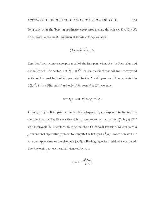
- Page 165: APPENDIX D. GMRES AND ARNOLDI ITERA


