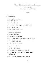
Abstract

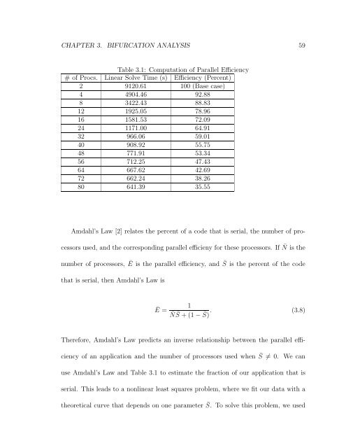
CHAPTER 3. BIFURCATION ANALYSIS 59
Table 3.1: Computation of Parallel Efficiency
#ofProcs. Linear Solve Time (s) Efficiency (Percent)
2 9120.61 100 (Base case)
4 4904.46 92.88
8 3422.43 88.83
12 1925.05 78.96
16 1581.53 72.09
24 1171.00 64.91
32 966.06 59.01
40 908.92 55.75
48 771.91 53.34
56 712.25 47.43
64 667.62 42.69
72 662.24 38.26
80 641.39 35.55
Amdahl’s Law [2] relates the percent of a code that is serial, the number of pro-
cessors used, and the corresponding parallel efficieny for these processors. If ¯ N is the
number of processors, Ē is the parallel efficiency, and ¯ S is the percent of the code
that is serial, then Amdahl’s Law is
Ē =
1
¯N ¯ S +(1− ¯ . (3.8)
S)
Therefore, Amdahl’s Law predicts an inverse relationship between the parallel effi-
ciency of an application and the number of processors used when ¯ S = 0. Wecan
use Amdahl’s Law and Table 3.1 to estimate the fraction of our application that is
serial. This leads to a nonlinear least squares problem, where we fit our data with a
theoretical curve that depends on one parameter ¯ S. To solve this problem, we used