Abstract

CHAPTER 2. TEMPORAL INTEGRATION 30
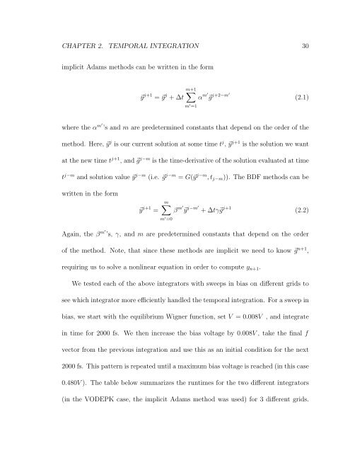
implicit Adams methods can be written in the form
y j+1 = y j +∆t
m+1
m ′ =1
α m′
g j+2−m′
(2.1)
where the αm′ ’s and m are predetermined constants that depend on the order of the
method. Here, y j is our current solution at some time t j , y j+1 is the solution we want
at the new time t j+1 ,andg j−m is the time-derivative of the solution evaluated at time
t j−m and solution value y j−m (i.e. g j−m = G(y j−m ,tj−m)). The BDF methods can be
written in the form
y j+1 =
m
m ′ =0
β m′
y j−m′
+∆tγg j+1
(2.2)
Again, the βm′ ’s, γ, andmare predetermined constants that depend on the order
of the method. Note, that since these methods are implicit we need to know g n+1 ,
requiring us to solve a nonlinear equation in order to compute yn+1.
We tested each of the above integrators with sweeps in bias on different grids to
see which integrator more efficiently handled the temporal integration. For a sweep in
bias, we start with the equilibrium Wigner function, set V =0.008V , and integrate
in time for 2000 fs. We then increase the bias voltage by 0.008V , take the final f
vector from the previous integration and use this as an initial condition for the next
2000 fs. This pattern is repeated until a maximum bias voltage is reached (in this case
0.480V ). The table below summarizes the runtimes for the two different integrators
(in the VODEPK case, the implicit Adams method was used) for 3 different grids.