Thermal properties in mesoscopics: physics and ... - ResearchGate
Thermal properties in mesoscopics: physics and ... - ResearchGate
Thermal properties in mesoscopics: physics and ... - ResearchGate

Create successful ePaper yourself
Turn your PDF publications into a flip-book with our unique Google optimized e-Paper software.
f N (E) (a)<br />
1<br />
0.8<br />
0.6<br />
0.4<br />
0.2<br />
0<br />
−0.6 −0.4 −0.2 0<br />
E/∆<br />
0.2 0.4 0.6<br />
f N (E)<br />
1<br />
0.8<br />
0.6<br />
0.4<br />
0.2<br />
K e−e =<br />
0<br />
1<br />
10<br />
100<br />
0<br />
−0.6 −0.4 −0.2 0<br />
E/∆<br />
0.2 0.4 0.6<br />
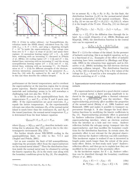
FIG. 6 (Color <strong>in</strong> onl<strong>in</strong>e edition): (a) Nonequilibrium distribution<br />
<strong>in</strong>side the SINIS isl<strong>and</strong>, calculated from Eq. (42)<br />
with Icoll = 0, T = 0.1Tc, <strong>and</strong> us<strong>in</strong>g a depair<strong>in</strong>g strength<br />
Γ = 10 −4 ∆ <strong>in</strong>side the superconductors. The voltage runs<br />
from zero to V = 3∆/e <strong>in</strong> steps of ∆/(2e) <strong>and</strong> spans three<br />
regimes: (i) anomalous heat<strong>in</strong>g regime (eV = 0 . . . ∆, solid<br />
l<strong>in</strong>es, widen<strong>in</strong>g with an <strong>in</strong>creas<strong>in</strong>g V ) discussed <strong>in</strong> (Pekola<br />
et al., 2004a), (ii) cool<strong>in</strong>g regime (eV = 1.5∆ <strong>and</strong> eV = 2∆,<br />
dashed l<strong>in</strong>es, narrow<strong>in</strong>g with an <strong>in</strong>creas<strong>in</strong>g V ) <strong>and</strong> the strong<br />
nonequilibrium heat<strong>in</strong>g regime (eV = 2.5∆ <strong>and</strong> eV = 3∆,<br />
dotted l<strong>in</strong>es, widen<strong>in</strong>g with an <strong>in</strong>creas<strong>in</strong>g V ). (b) Distribution<br />
at eV = 2.5∆ for different strengths of the electron–<br />
electron <strong>in</strong>teraction, parametrized by the parameter Ke−e<br />
from Eq. (16) with RD replaced by RT <strong>and</strong> E ∗ by ∆, as<br />
<strong>in</strong> this case these describe the collision <strong>in</strong>tegral.<br />
performance at the lowest temperatures, <strong>and</strong> to overheat<br />
the superconductor at the junction region due to strong<br />
power <strong>in</strong>jection. Barrier optimization <strong>in</strong> terms of both<br />
materials <strong>and</strong> technology seems to be still nowadays a<br />
challeng<strong>in</strong>g task (see also Sec. VI.F.1).<br />
In a SINIS system <strong>in</strong> the quasiequilibrium limit, the<br />
temperatures Te,N <strong>and</strong> Te,S of the N <strong>and</strong> S parts may<br />
differ. If the superconductors are good reservoirs, Te,S<br />
equals the lattice temperature. In the experimentally<br />
relevant case when the resistance RD of the normal-metal<br />
isl<strong>and</strong> is much lower than the resistances RL <strong>and</strong> RR of<br />
the tunnel junctions, the normal-metal temperature Te,N<br />
is determ<strong>in</strong>ed from the heat balance equation<br />
(b)<br />
˙QSINIS(V ; Te,S, Te,N ) = Pcoll, (40)<br />
where ˙ QSINIS = 2 ˙ QNIS <strong>and</strong> Pcoll describes <strong>in</strong>elastic scatter<strong>in</strong>g<br />
due to phonons (Eq. (24)) <strong>and</strong>/or due to the electromagnetic<br />
environment (Eq. (25)).<br />
For further details about NIS/SINIS cool<strong>in</strong>g <strong>in</strong> the<br />
quasiequilibrium limit, we refer to Sec. V.C.1 <strong>and</strong><br />
(Anghel <strong>and</strong> Pekola, 2001).<br />
Let us now consider the limit of full nonequilibrium,<br />
neglect<strong>in</strong>g the proximity effect from the superconductors<br />
on the normal-metal isl<strong>and</strong>. 2 Then the distribution function<br />
<strong>in</strong>side the normal metal may be obta<strong>in</strong>ed by solv<strong>in</strong>g<br />
the k<strong>in</strong>etic equation Eq. (3) <strong>in</strong> the static case along with<br />
the boundary conditions given by Eq. (8). For simplicity,<br />
2 This is justified <strong>in</strong> the limit RL, RR ≫ RD.<br />
12<br />
let us assume RL = RR ≡ RT ≫ RD. In this limit, the<br />
distribution function fN (E) <strong>in</strong> the normal-metal isl<strong>and</strong><br />
is almost <strong>in</strong>dependent of the spatial coord<strong>in</strong>ate. Then,<br />
<strong>in</strong> Eq. (3) we can use ∂ 2 xf ≈ (∂xf(L) − ∂xf(0))/L, where<br />
L is the length of the N wire. From Eq. (11) we then get<br />
RD<br />
RT<br />
(NR(fN − fR) − NL(fL − fN)) = τDIcoll, (41)<br />
where τD = L2 N /D is the diffusion time through the isl<strong>and</strong>.<br />
As a result (Giazotto et al., 2004b; Hesl<strong>in</strong>ga <strong>and</strong><br />
Klapwijk, 1993), the distribution function <strong>in</strong> the central<br />
wire can be expressed as<br />
fN = fRNR + fLNL + RIVe 2νF Icoll<br />
. (42)<br />
NR + NL<br />
Here V = LA is the volume of the isl<strong>and</strong>. In the presence<br />
of <strong>in</strong>elastic scatter<strong>in</strong>g, this is an implicit equation, as Icoll<br />
is a functional of fN . Examples of the effect of <strong>in</strong>elastic<br />
scatter<strong>in</strong>g have been considered <strong>in</strong> (Hesl<strong>in</strong>ga <strong>and</strong> Klapwijk,<br />
1993) <strong>in</strong> the relaxation time approach, <strong>and</strong> <strong>in</strong> (Giazotto<br />
et al., 2004b) <strong>in</strong>clud<strong>in</strong>g the full electron–electron<br />
scatter<strong>in</strong>g collision <strong>in</strong>tegral. The distribution function<br />
fN <strong>in</strong> Eq. (42) is plotted <strong>in</strong> Fig. 6 for a few values of the<br />
voltage for Icoll = 0 <strong>and</strong> for a few strengths of electron–<br />
electron scatter<strong>in</strong>g at eV = 2.5∆.<br />
3. Superconductor-normal-metal structures with transparent<br />
contacts<br />
If a superconductor is placed <strong>in</strong> a good electric contact<br />
with a normal metal, a f<strong>in</strong>ite pair<strong>in</strong>g amplitude is <strong>in</strong>duced<br />
<strong>in</strong> the normal metal with<strong>in</strong> a thermal coherence<br />
length ξT = D/(2πkBT ) near the <strong>in</strong>terface. This<br />
superconduct<strong>in</strong>g proximity effect modifies the <strong>properties</strong><br />
of the normal metal (Belzig et al., 1999; Lambert <strong>and</strong><br />
Raimondi, 1998) <strong>and</strong> makes it possible to transport supercurrent<br />
through it. It also changes the local distribution<br />
functions by modify<strong>in</strong>g the k<strong>in</strong>etic coefficients <strong>in</strong><br />
Eq. (5). Superconduct<strong>in</strong>g proximity effect is generated<br />
by Andreev reflection (Andreev, 1964b) at the normalsuperconduct<strong>in</strong>g<br />
<strong>in</strong>terface, where an electron scatters<br />
from the <strong>in</strong>terface as a hole <strong>and</strong> vice versa. Andreev<br />
reflection forbids the sub-gap energy transport <strong>in</strong>to the<br />
superconductor, <strong>and</strong> thus modifies the boundary conditions<br />
for the distribution functions. In certa<strong>in</strong> cases, the<br />
proximity effect is not relevant for the physical observables<br />
whereas the Andreev reflection can still contribute.<br />
This <strong>in</strong>coherent regime is realized if one is <strong>in</strong>terested <strong>in</strong><br />
length scales much longer than the extent of the proximity<br />
effect. Below, we first study such ”pure” Andreevreflection<br />
effects, <strong>and</strong> then go on to expla<strong>in</strong> how they are<br />
modified <strong>in</strong> the presence of the proximity effect.<br />
In the <strong>in</strong>coherent regime, for E < ∆, Andreev reflection<br />
can be described through the boundary conditions<br />
(Pierre et al., 2001)<br />
f(µS + E) = 1 − f(µS − E) (43a)<br />
ˆn · ∇[f(µS − E) − f(µS + E)] = 0, (43b)