Geological Survey of Denmark and Greenland Bulletin 26 ... - Geus

A
Basement
A
Skaergaard intrusion
68°11´N
B
31°43´W
B
C
Fig. 2. Simplified workflow diagram describing the process of generating
3D data from photographs to 3D modelling. A: polylines representing
geological boundaries or structures are extracted from a 3D stereo plotter.
B: The nodes of the polylines are converted into structural readings (here
shown as small blue discs) using the GEUS Planes tool. Measurements with
a poorly defined plane (high standard deviation on either the dip, dip-azimuth
or plane) are discarded. C: The structural readings are imported into
a 3D modelling software (Leapfrog 3D) where surfaces and volumes can be
generated and compiled to a 3D model of the geological object.
1 km
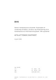
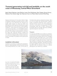
Fig. 3. Example of a polyline (blue) representing the boundary between
the Skaergaard intrusion (dark grey in Fig. 3A, light yellow to red in Fig.
3B, representing different lithological units) and the basement (light
grey in Fig. 3A, light skin tone in Fig. 3B). The same polyline is drawn
on the 1:27 000 aerial photographs (A) and shown on the geological map
of McBirney (1989) (B) for comparison. The difference between the locations
of the two lines is up to 100 m.
58