Geological Survey of Denmark and Greenland Bulletin 26 ... - Geus

A spectrogram produced by short-time Fourier transform
is a very useful tool in seismology because it can provide an
image indicating the time at which a burst of energy occurs
on a seismogram, in addition to the spectral composition of
the signal (Gibbons et al. 2008). The event detection algorithm
used in this study inspects the temporal variation of
the signal spectrogram calculated in frequency bands corresponding
to the frequency content of local and regional
earthquakes (e.g. 2–16 Hz). For detected events, the P- and
S-phases are picked. An example of a recorded seismogram
with an earthquake signal and corresponding spectrogram
is shown in Fig. 2 where an earthquake is observed on a seismogram
at an approximate time of 800 s. Obvious changes
in the colour of the spectrogram take place over a wide range
of frequencies along the time axis, which indicate the arrivals
of earthquake energy (Fig. 2B). Accordingly, the detection
of a change in energy pattern over a pre-defined range of
frequencies, corresponding to the frequency content of the
earthquake signals, leads to the detection of an earthquake.
The plots presented in Fig. 2C show the variation of energy
for each frequency band, corresponding to the above spectrogram.
These plots provide another representation of the
spectrogram. The problem of detecting an earthquake on
seismograms is now reduced to detecting sharp increases in
the individual time series representing spectral energy versus
time (the plot shown in Fig. 2C). To avoid false detections
due to seismic noise with a frequency content overlapping
the analysed frequencies, only detections made in most of
the frequency bands are accepted. For instance, detections
should be made at about the same time in at least five out of
eight frequency sub-bands for a given spectrogram (Fig. 2B).
Three missing detections are allowed, because this may happen
for small events and noisy backgrounds, or low signal to
noise ratio in some frequency bands. To reduce the false detection
rate, all three components (vertical, N–S and E–W)
of the seismograms are used in the event detection procedure.
Results
To test the automatic detection method, Station Nord data
from 6 July 2010 to 6 March 2011 were used. Prior to this
period, the digitising unit of the seismometer had been upgraded
to sample at 100 Hz. Earlier, the instrument had sampled
at 20 Hz; this limits earthquake analysis to frequencies
below 10 Hz, which the automatic method was not prepared
for. Station Nord is equipped with a Streckeisen STS-2 sensor
and a Quanterra Q330 digitiser. The automatic method
analyses data from all three components of the sensor, using
24 hour data files. The data are band pass filtered between
0.95 and 20 Hz before the detection algorithm is applied. The
Plot start 10 Feb. 2011 4:52:15.000
Vertical component
North–south component
East–west component
A
Duration
Filter: 1–17 Hz
Time (min.; UTC)
04:53 04:54 04:55 04:56 04:57 04:58
Plot start 26 Sep. 2010 10:15:59.320
Vertical component
Vertical component
P
S
S
P
Filter: 1–17 Hz
Time (min.; UTC)
10:17 10:18 10:19 10:20 10:21
Filter: 2–9 Hz
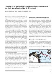
Fig. 3. A: Seismogram of a magnitude 2.2 earthquake filtered with a 1–17
Hz band pass filter containing the frequencies used for the automatic detection.
The epicentre was located 354 km south-south-east of Station
Nord. The automatic P-phase (P) was kept in the review, but the automatic
S-phase (S) was repicked moving the epicentre 118 km. Automatic S pick
is seen on the north–south channel, manual S pick is seen on the east–west
channel and the automatic tremor duration is seen on the vertical channel.
B: Vertical component of an earthquake not detected by the automatic
method. Top trace: data with the 1–17 Hz filter used by the automatic
method. Bottom trace: data with the 2–9 Hz filter used by the manual
method. The earthquake had a magnitude of 1.1 and was located 234 km
east-south-east of Station Nord. UTC: Universal Time, Coordinated.
B
79