PHYS08200604017 Manimala Mitra - Homi Bhabha National Institute

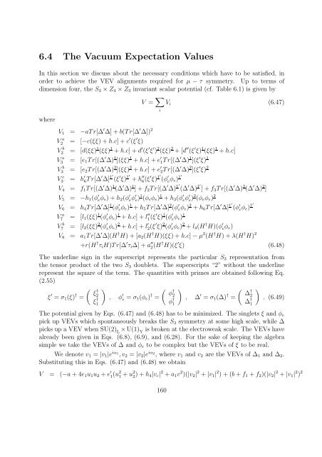
6.4 The Vacuum Expectation Values
In this section we discuss about the necessary conditions which have to be satisfied, in
order to achieve the VEV alignments required for µ − τ symmetry. Up to terms of
dimension four, the S 3 ×Z 4 ×Z 3 invariant scalar potential (cf. Table 6.1) is given by
V = ∑ i
V i (6.47)
where
V 1 = −aTr[∆ ′ ∆]+b(Tr[∆ ′ ∆]) 2
V2 a = [−c(ξξ)+h.c]+c ′ (ξ ′ ξ)
V2 b = [d(ξξ) 1 (ξξ) 1 +h.c]+d ′ (ξ ′ ξ ′ ) 2 (ξξ) 2 +[d ′′ (ξ ′ ξ) 1 (ξξ) 1 +h.c]
V3 a = [e 1 Tr[(∆ ′ ∆) 1 ](ξξ) 1 +h.c]+e ′ 1 Tr[(∆′ ∆) 1 ](ξ ′ ξ) 1
V3 b = [e 2 Tr[(∆ ′ ∆) 2 ](ξξ) 2 +h.c]+e ′ 2Tr[(∆ ′ ∆) 2 ](ξ ′ ξ) 2
V3 c = h ′ 6 Tr[∆′ ∆] 1′ (ξ ′ ξ) 1′ +h ′′
6 (ξ′ ξ) 1′ (φ ′ e φ e) 1′
V 4 = f 1 Tr[(∆ ′ ∆) 1 (∆ ′ ∆) 1 ]+f 2 Tr[(∆ ′ ∆) 1′ (∆ ′ ∆) 1′ ]+f 3 Tr[(∆ ′ ∆) 2 (∆ ′ ∆) 2 ]
V 5 = −h 1 (φ ′ eφ e )+h 2 (φ ′ eφ ′ e) 1 (φ e φ e ) 1 +h 3 (φ ′ eφ ′ e) 2 (φ e φ e ) 2
V 6 = h 4 Tr[∆ ′ ∆] 1 (φ ′ e φ e) 1 +h 5 Tr[∆ ′ ∆] 2 (φ ′ e φ e) 2 +h 6 Tr[∆ ′ ∆] 1′ (φ ′ e φ e) 1′
V a
7 = [l 1 (ξξ) 1 (φ ′ e φ e) 1 +h.c]+l ′′
1 (ξ′ ξ) 1 (φ ′ e φ e) 1
V b
7 = [l 2 (ξξ) 2 (φ ′ eφ e ) 2 +h.c]+l ′ 2(ξ ′ ξ) 2 (φ ′ eφ e ) 2 +l 4 (H † H)(φ ′ eφ e )
V 8 = a 1 Tr[∆ ′ ∆](H † H)+[a 2 (H † H)(ξξ)+h.c]−µ 2 (H † H)+λ(H † H) 2
+r(H † τ i H)Tr[∆ ′ τ i ∆]+a ′′
2 (H† H)(ξ ′ ξ) (6.48)
The underline sign in the superscript represents the particular S 3 representation from
the tensor product of the two S 3 doublets. The superscripts “2” without the underline
represent the square of the term. The quantities with primes are obtained following Eq.
(2.55)
ξ ′ = σ 1 (ξ) † =
(
ξ
†
2
ξ † 1
)
, φ ′ e = σ 1 (φ e ) † =
(
φ
†
2
φ † 1
)
, ∆ ′ = σ 1 (∆) † =
(
∆
†
2
∆ † 1
)
. (6.49)
The potential given by Eqs. (6.47) and (6.48) has to be minimized. The singlets ξ and φ e
pick up VEVs which spontaneously breaks the S 3 symmetry at some high scale, while ∆
picks up a VEV when SU(2) L
×U(1) Y
is broken at the electroweak scale. The VEVs have
already been given in Eqs. (6.8), (6.9), and (6.28). For the sake of keeping the algebra
simple we take the VEVs of ∆ and φ e to be complex but the VEVs of ξ to be real.
We denote v 1 = |v 1 |e iα 1
,v 2 = |v 2 |e iα 2
, where v 1 and v 2 are the VEVs of ∆ 1 and ∆ 2 .
Substituting this in Eqs. (6.47) and (6.48) we obtain
V = (−a+4e 1 u 1 u 2 +e ′ 1 (u2 1 +u2 2 )+h 4|v c | 2 +a 1 v 2 )(|v 2 | 2 +|v 1 | 2 )+(b+f 1 +f 2 )(|v 2 | 2 +|v 1 | 2 ) 2
160