Report PDF (3.7 MB) - USGS

More documents

Recommendations

Info

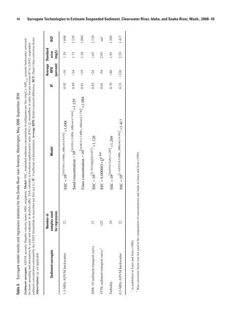
14 Surrogate Technologies to Estimate Suspended Sediment, Clearwater River, Idaho, and Snake River, Wash., 2008–10 Table 3. Surrogate model results and regression statistics for the Snake River near Anatone, Washington, May 2008–September 2010. [Sediment surrogate: ADVM, acoustic Doppler velocity meter; MHz, megahertz. Model: SSC, suspended-sediment concentration in milligrams per liter (mg/L); ABS corr , acoustic backscatter corrected for beam spreading and attenuation by water and sediment in decibels (dB); Turb, turbidity in Formazin nephelometric units (FNU); Q, streamflow in cubic feet per second (ft 3 /s); LISST, suspendedsediment concentration estimated by the LISST StreamSide in microliter per liter (µL/L). R 2 : Coefficient of determination. Average RPD: Relative percent difference. BCF: Duan’s bias correction factor. Abbreviation: na, not applicable Sediment surrogate Number of samples used for regression Model R 2 RPD Average (percent) Standard error (mg/L) BCF 1.5-MHz ADVM backscatter 22 ⎡( 0.0756 × 1.5-MHz_ABScorr ) -4.676 ⎤ SSC = 10 ⎣ ⎦ × 1.048 0.92 +10 1.39 1.048 ⎡( 0.105 × 1.5-MHz_ABScorr ) -7.636 Sand concentration = 10 ⎣ ⎤⎦ × 1.129 0.89 +24 1.73 1.129 ⎡( 0.0615 × 1.5-MHz_ABScorr ) -<strong>3.7</strong>30 Fines concentration = 10 ⎣ ⎤⎦ × 1.084 0.81 +19 1.54 1.084 ⎡ 2008–10 sediment transport curve 33 ( 1.761 × log ( Q ) ) -6.697 ⎤ SSC = 10 ⎣ ⎦ × 1.120 0.83 +24 1.65 1.120 1970s sediment transport curve 1 125 1.460 SSC = 0.000003 × Q 0.61 -34 2.03 na 2 Turbidity 29 ⎡( 0.0181 Turb ) 1.249 SSC 10 × + ⎤ = ⎣ ⎦ × 1.209 0.70 +48 1.93 1.209 0.5-MHz ADVM backscatter 22 ⎡( 0.0333 0.5-MHz_ABScorr ) 4.301 SSC 10 − × + ⎤ = ⎣ ⎦ × 1.417 0.33 +120 2.59 1.417 1 As published in Jones and Seitz (1980). 2 Bias correction factor was not used in the computation of concentrations and loads in Jones and Seitz (1980).
Use of Surrogate Models To Estimate Suspended Sediment 15 The model between 0.5 MHz acoustic backscatter and SSC was poor (R 2 =0.007) because of a problem noted in the instrument noise level measurements. At high flows, the measured noise level increased substantially and was high relative to the raw backscatter measurement. The 0.5-MHz ADVM appears to be more sensitive to electrical and other noise that occurs in the water at high streamflows than the other evaluated frequencies (Craig Huhta, SonTek/Yellow Springs Instruments, oral commun., 2012). Because the instrument noise level is subtracted from the raw backscatter to compute SNR, in many cases this resulted in a low SNR when SSC was high. For comparison, a model was developed between the raw backscatter from the 0.5-MHz ADVM (without subtracting the noise level) and SSC, resulting in an improved R 2 of 0.89, but raw backscatter data collected during this period also could have been erroneous. Overall, the 3-MHz ADVM was still a better estimator of SSC than the other surrogates whether raw backscatter or SNR was used to develop the model. Topping and others (2004) determined that in the Colorado River, the degree of sediment attenuation along the beam path is closely related to the fines fraction, and average backscatter is closely related to the sand fraction. However, backscatter alone was determined to be a good estimator of the fines and sand fractions, as well as overall SSC, in the Clearwater River. The model between 3-MHz acoustic backscatter and SSC (overall, sand, and fines) shows that a shift from a fines-dominated SSC to a sand-dominated SSC occurs around 60 mg/L or an ABS corr for the 3-MHz ADVM of 75 dB (fig. 5). Non-zero attenuation at low SSC, likely because of the presence of organic matter, created significant variability in the relation between attenuation and the fines fraction, as well as overall SSC, at low concentrations. High variability in the individual sand and fines models is caused by many physical factors of sediment load and transport including the magnitude of the washload component, mobility of bed material and armor, non-equilibrium (supply limited) transport 2.5 EXPLANATION 2.0 Total suspended-sediment concentration Sand concentration Fines concentration Log suspended-sediment concentration, in log milligrams per liter 1.5 1.0 0.5 0.0 0.5 Total suspended sediment log SSC = (0.0557 × 3-MHz_ABS corr )−2.431 R² = 0.93 Sand log Sand = (0.0743 × 3-MHz_ABS corr )−4.147 R² = 0.87 Fines log Fines = (0.0461 × 3-MHz_ABS corr )−2.030 R² = 0.78 1.0 50.0 55.0 60.0 65.0 70.0 75.0 80.0 85.0 Sediment- and water-corrected acoustic backscatter (ABS corr ) from 3-Megahertz (MHz) acoustic Doppler velocity meter (ADVM), in decibels Figure 5. Surrogate regression models for total suspended sediment, sand, and fines concentrations based on acoustic backscatter for the Clearwater River near Spalding, Idaho.
Page 1 and 2: Prepared in cooperation with the U.
Page 3 and 4: Use of Surrogate Technologies to Es
Page 5 and 6: iii Contents Abstract .............
Page 7 and 8: v Conversion Factors and Datums Con
Page 9 and 10: Use of Surrogate Technologies to Es
Page 11 and 12: Introduction 3 The Lower Granite Lo
Page 13 and 14: Site Descriptions and Surrogate Ins
Page 15 and 16: Site Descriptions and Surrogate Ins
Page 17 and 18: Methods 9 Surrogate Instrument Data
Page 19 and 20: Methods 11 Acoustic Absorption by S
Page 21: Use of Surrogate Models To Estimate
Page 25 and 26: Use of Surrogate Models To Estimate
Page 35 and 36: References Cited 27 Summary and Con
Page 37 and 38: References Cited 29 SonTek/Yellow S
Page 39 and 40: Publishing support provided by the

Report PDF (3.7 MB) - USGS

Create successful ePaper yourself

Delete template?

Save as template?