EDAX EDS Manual

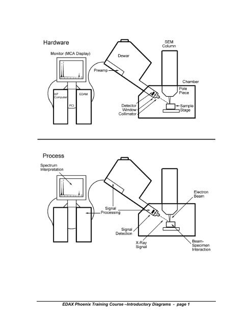
EDAX Phoenix Training Course –Introductory Diagrams - page 1

ENERGY DISPERSIVE X-RAY SPECTROMETRY--
EDS INSTRUMENTATION & SIGNAL DETECTION
1. X-Ray Detectors:
ALAN SANDBORG
EDAX INTERNATIONAL, INC.
The EDS detector is a solid state device designed to detect x-rays and convert their
energy into electrical charge. This charge becomes the signal which when processed
then identifies the x-ray energy, and hence its elemental source.
The X-ray in its interaction with solids, gives up its energy and produces electrical
charge carriers in the solid. A solid state detector can collect this charge. One of the
desirable properties of a semiconductor is that it can collect both the positive and
negative charges produced in the detector. The figure below shows the detection
process.
Figure 1.
There are two types of semiconductor material used in electron microscopy. They are
silicon (Si) and germanium (Ge). In Si, it takes 3.8 eV of x-ray energy to produce a
charge pair, and in Ge it takes only 2.96 eV of energy. The other properties of these two
types will be discussed later in this section. The predominant type of detector used is
the Si detector, so it will be favored in the discussions. With a Si detector, an O K x-ray
whose energy is 525eV will produce 525/3.8= 138 charge pairs. A Fe K x-ray will
produce 6400/3.8= 1684 charge pairs. So by collecting and measuring the charge, the
EDAX Phoenix Training Course - EDS Instrumentation & Signal Detection - page 1

Important EDS Parameters
Count Rate
For a good quality spectrum (i.e. good resolution and fewest artifacts) you should use the
50 or 100 us time constant (pulse processing time) with a deadtime of 20 to 40%, and 500
to 2500 cps.These are good numbers if the sample consists largely of high energy peaks (>
1 keV), but if the spectrum is dominated by low energy peaks (< 1 keV) then a count rate of
500 - 1000 cps is better and the 100 us time constant should be used.
When maximum count throughput is required, such as when collecting fast x-ray maps, a
faster time constant (2.5 to10 us) should be used with a count rate of 10,000 to 100,000
cps. The deadtime should not exceed 50 to 67%. These conditions may not be optimum for
low energy peaks in terms of their resolution and/or position. A lower count rate and slower
time constant should be and/or it might be necessary to adjust the position of the ROI prior
to collecting the map.
Accelerating Voltage
The overvoltage is a ratio of accelerating voltage used to the critical excitation energy of a
given line for an element. Typically, the overvoltage should be at least 2 for the highest
energy line and no more than 10 to 20 times the lowest energy line of interest. We use the
number 10 for quantitative applications and the 20 for qualitative applications.
For example, if you are interested in analysis of a phase containing Fe, Mg and Si and want
to use the K lines for each, then 15 kV will probably work reasonably well. If, however, you
need to analyze the same three elements plus oxygen as well, then you might use 5 to 10
kV, but you might want to use the L line for the Fe.
Why should the overvoltage be at least 2 for the highest energy element? Because at lower
overvoltages the fraction of the interaction volume where the element can be excited
becomes very small and you will not be able to generate very many x rays of that energy.
Why should the overvoltage be less than 10 to 20 times the lowest energy peak? When the
overvoltage number is excessive, the proportion of the interaction volume for which the low
energy x rays can escape without being absorbed also becomes small. The result is a
small peak and in the case of the quantification there will be a strong absorption correction
which will magnify the statistical errors in our analysis.
Take-Off Angle
Typical take-off angles will range from 25 to 40 degrees. This angle is a combination of the
detector angle, its position, sample working distance and sample tilt. The sensitivity for very
low energy x rays and/or signals characterized by high absorption can be enhanced by
increasing the take-off angle. Some inclined detectors (e.g. a detector angle of
approximately 35 degrees above the horizontal) do not require sample tilt. Horizontal entry
detectors require that the sample be tilted to achieve an optimum take-off angle.
EDAX Phoenix Training Course - EDS Parameters - page 1

EDAX Detector Geometry
The elevation angle (EA) is the angle
between the horizontal and the detector
normal. The intersection distance (ID) is the
distance in mm between the pole piece
where the electron beam intersects the
detector normal. The azimuth angle can not
be shown in a cross-sectional view as
shown at the left, but it is the angle as
viewed from above between the detector
normal and normal to the tilt axis. The
working distance (WD) is where the sample
is in mm below the pole piece. The take-off
angle (TOA) is the angle between the x-ray trajectory and the sample surface. If the sample is
placed at the intersection distance and not tilted, the take-off angle will equal the elevation angle.
If the working distance is shorter than
the intersection distance, the take-off
angle will be less than the elevation
angle. This assumes that the sample is
smooth and not tilted.
If the working distance is longer than
the intersection distance, the take-off
angle will be more than the elevation
angle. Again, this assumes that the
sample is smooth and not tilted.
If the sample is tilted toward the detector,
the take-off angle will be greater
than the elevation angle. If the sample
were tilted away from the detector, the
take-off angle would be less than the
elevation angle. Note that the azimuth
angle must be taken into account to
determine the take-off angle.
EDAX Phoenix Training Course - EDAX Detector Geometry - page 1

Dead Time & Time Constants
In an EDS system the real time (or clock time) is divided into live time and dead time. The
live time is the time when the detector is alive and able to receive an x-ray event (i.e. the
time when it is doing nothing) and the dead time is when the detector or preamplifier is
unable to accept a pulse because it is busy processing or rejecting an event(s). Basically,
the charges from an x-ray photon can be collected in about 50 ns and in the end we will take
roughly 50 us to process the filtered, amplified pulse (1000 times longer). Quite often, x-ray
photons will come in too close to each other and we will reject the signals. That is why we
can see the situation that we actually collect very few x-ray events at very high count rates
and we actually process more counts when we use a lesser count rate.
If we decide to take less time to process the pulse in the end (say, less than a 10 us time
constant or pulse processing time) then we can process more counts. However, because
we have taken less time, there is the possibility that we do not process the peak energy as
accurately and the peaks will be broader; the resolution will be poorer or higher.
The Phoenix system has 8 time constants or pulse processing times which will allow for
optimum resolution or x-ray count throughput. Under most circumstances, we would like to
have a dead time that is between 10 and 40% and perhaps between 20 and 30% if we would
like to tighten the range of our analytical conditions. There are times when we are most
concerned about the count throughput and are not concerned about resolution, sum peaks,
etc., such as when we are collecting x-ray maps. Under these conditions a dead time as
high as 50 to 60% is feasible. Under no circumstances should a dead time that is more than
67% be used because we will actually get fewer counts processed.
A series of plots are included on the following pages. These show: the fall-off in processed
counts when the count rate is increased too high, a comparison in throughput between a fast
time constant and a slower time constant, and a plot showing the dead time % for various
count rates and time constants, and a plot of count rate versus dead time % for each of the 8
time constants.
EDAX Phoenix Training Course –Dead Time & Time Constants - page 1

EDX SPECTRUM INTERPRETATION AND ARTIFACTS
Continuum X Rays
As a result of inelastic scattering of the primary beam electrons in which the electrons
are decelerated and lose energy without producing an ionization of the atoms in the
sample, continuum x rays are formed. The continuum x rays are the background of our
EDS spectrum and are sometimes referred to as the bremsstrahlung. In theory, the
continuum can be expected to extend from the maximum energy of the primary beam
electrons and increase exponentially to zero keV energy. In reality, the background
goes to zero at the low end of the energy spectrum due to absorption by the detector
window, the detector dead layer, and the gold layer. The intensity of the continuum is
related to both the atomic number of the sample as well as the beam energy. The
continuum intensity also increases with beam current.
Characteristic X Rays
Inelastic scattering events between the primary beam electrons and inner shell electrons
which result in the ejection of the electron from the atom within the sample and may lead
to the formation of a characteristic x ray. The ejection of the electron leaves the atom in
an ionized, excited state and permits an outer shell electron to move to the inner shell.
Because the energy levels of the various shells are related to the number of charges in
the nucleus, the energy of the emitted x ray is “characteristic” of the element. The beam
electron must have an energy greater that is just slightly greater than the energy of the
shell electron (the critical ionization energy).
Depth of Excitation
Although electrons may penetrate to specific depths within a sample which can be
illustrated with a variety of equations or with Monte Carlo programs, the electrons
actually lose energy in steps as they go to greater depths in the sample. As a result, an
electron may soon lose a sufficient amount of its energy such that it can no longer excite
characteristic x rays. Typically, this occurs when its energy drops below the critical
ionization energy of the elements in the sample. Each element within the sample will
have its own critical ionization energy and its own excitation depth. The ratio of the
primary beam energy to the excitation energy of the element is referred to as the
EDAX Phoenix Training Course - Spectrum Interpretation & Artifacts - page 1

EDAX Phoenix Peak Identification
The basic procedure for identifying peaks in the EDS spectrum is not always agreed upon.
Some users start with the biggest peak, identify it and all associated peaks, and then
progress to the smaller peaks in sequence until all are identified. When there are L- and Mseries
peaks present, it may actually be better to identify the highest energy alpha peak first
because this peak may be associated with several other higher energy peaks as well as one
or more of the lower energy peaks. Then, the user can find the next lowest energy peak,
etc., until all peaks have been accounted for. Another significant aid for peak ID is to click
on the button for the automatic peak ID. The results of the automatic peak ID should be
inspected and verified; it very often will provide the correct answer, but the user should be
aware that its answer might be only a part of the solution and that more investigation may be
required. In all cases, however, it is essential to look for escape peaks for the peaks of
greatest height and for sum peaks for these same peaks when a high count rate has been
used for spectrum acquisition.
Typically, we examine that part of the spectrum that ranges in energy between 0 and 10 keV
and we quickly become aware of characteristic features of K-, L- and M-shell x-ray peaks
that aid us in our peak identification. In this energy range, we can see peaks with K-shell xrays
that correspond to atomic numbers 4 through 32, L-shell peaks that range from roughly
atomic numbers 22 to 79, and M-shell x rays ranging from 56 to the highest known and
observable atomic numbers. For many elements it is possible to observe peaks from more
than one shell in this energy range (it is often desirable to inspect the region between 10 and
20 keV as well for confirmation of lower energy peaks). The resolution of the peak of one
element from an adjacent atomic number is often better resolved by using higher energy
peaks (see spectrum of Ni and Cu below).
EDAX Phoenix Training Course - Peak ID - page 1

EDAX Peak ID Quiz –“sp_pkid” Spectra
On the floppy disk provided with this notebook is a directory “sp_pkid”. This directory
contains a series of spectra “pkidXX.spc” and “deconXX.spc”. The spectra pkid01 through
pkid04 and pkid06 are the same spectra used for illustrations in the “Peak Identification”
discussion. Other spectra on the disk can be used as a peak identification quiz and they
range in difficulty from relatively easy to impossible. In the space below, identify the peak by
element and shell (e.g. SiK, PbM, SnL, etc.).
Quiz:
PkID05.spc (easy). Between 1.5 and 12 keV, the peaks are:
PkID05b.spc (easy). Between 3.7 and 7.5 keV, the peaks are:
PkID07.spc (moderately hard). Between about 0.9 and 18 keV, the peaks are:
PkID08.spc (moderate). Between 0.6 and 14 keV, the peaks are:
PkID09.spc (hard). Between 0.55 and 15 keV, the peaks are:
PkID10.spc (easy to moderate). Between 0.2 and 10 keV, the peaks are:
Peak ID Quiz -- page 1

EDAX Peak ID Quiz –“sp_pkid” Spectra
On the floppy disk provided with this notebook is a directory “sp_pkid”. This directory
contains a series of spectra “pkidXX.spc” and “deconXX.spc”. The spectra pkid01 through
pkid04 and pkid06 are the same spectra used for illustrations in the “Peak Identification”
discussion. Other spectra on the disk can be used as a peak identification quiz and they
range in difficulty from relatively easy to impossible.
Quiz Answers:
PkID05.spc. This spectrum shows a series of K-series peaks with atomic numbers 14, 16,
18, 20, 22, 24, 26, 28, 30, and 32 (Si, S, Ar, Ca, Ti, Cr, Fe, Ni, Zn, Ge). There is good
separation of the Ka peaks and the Kb peaks are easily seen. The L-series peaks are not so
well resolved.
PkID05b.spc. A similar spectrum to PkID05 except that this shows a K-series peak for every
atomic number between 21 and 27 (Sc, Ti, V, Cr, Mn, Fe, and Co). In this area of the
spectrum the Kb peak of a given atomic number is overlapped by the Ka of the next higher
atomic number. Note the non-resolution of the L-series peaks for the same atomic numbers.
PkID07.spc. This spectrum is an older, non-Sapphire spectrum; that is why you will get the
dialog box asking if you want to “ignore”, “cancel” etc. From 1 keV to 18 keV, the peaks
present are:
ZnL, (NaK?), MgK, AlK + BrL, Si, NbL (probable), MoL, ClK, K K, TiK, V K, CrK, MnK,
FeK, CoK, NiK, CuK, ZnK, BrK, MoK.
PkID08.spc. Between 0.6 and 14 keV, the peaks are:
NiL, SeL, ZrL, PdL, TeL, TiK, NiK, SeK.
PkID09.spc. Between 0.55 and 15 keV, the peaks are:
F K, TaM, ThM, TaL, ThL. (This spectrum might also have some Uranium and other
radioactive elements).
PkID10.spc. Between 0.2 and 10 keV, the peaks are:
C K, CrL, NiL AlK, SiK, MoL, TiK, CrK, FeK, CoK, NiK. (There is probably also some
CoL in the sample but it is not a resolved peak).
PkID11.spc. Between 1 and 10 keV, the peaks are:
P K, InL.
PkID12.spc. Between 1 and 10 keV, the peaks are:
S K, CdL.
Decon01.spc. Between 1 and 10 keV, the peaks are (or might be):
IrM, P K, ZrL, InL, IrL.
Decon01b.spc. Between 1 and 10 keV, the peaks are (or might be):
Y L (?), IrM, P K (?), ZrL (?), InL, SnL, IrL.
EDAX Quiz on Peak ID - page 1

THE OPTIMIZATION OF X-RAY COUNT THROUGHPUT
The x-ray count rate is certainly one our most fundamental parameters for determining
optimal spectrum conditions. It is counter-intuitive for most users that increasing the
count rate does not automatically result in a better spectrum or at a minimum in
collecting more counts. The EDAX detector amplifier has two time constants (20 µs and
40 µs) which control the amount of time taken to process an x-ray event. While the x
ray is being processed, the detector is “dead” and will not process any additional events.
For each time constant there is a maximum throughput. When it is desirable to have
more counts in a spectrum or in a map, it is always possible to collect the signal for a
longer interval of time, but it is also possible to use a shorter time constant. When the
shorter time constant is employed, the spectrum resolution degrades but for many
applications this is not a serious drawback.
The figure below provides an example of how many counts can be processed in a fixed
interval of time (20 clock seconds). With the longer time constant (“40 tc” or 40 µs),
there are actually fewer counts processed when the count rate was increased from 2000
to 10,000 cps. The same 10,000 cps count rate yielded 6 to 7 times more processed
counts when the shorter time constant (“20 tc” or 20 µs). With the shorter time constant,
doubling the count rate only increased the processed counts by about ¼.
The resolution of the detector degrades noticeably when using the longer time constant
(see figure on the next page), but resolution is not normally a fundamental concern
when we do certain procedures such as collecting x-ray maps, or when the spectra
collected do not have significant overlaps and we are not concerned with low-energy
peaks or their analysis.
EDAX Training Course - X-Ray Count Optimization - page 1

SEM QUANT ZAF
Geometry
� The EDX detector parameters are specific for each microscope. The
elevation angle, intersection distance, azimuth angle, and scale
setting must be known and understood for microscope/detector
geometry. Before collecting a spectrum, an accurate accelerating
voltage should be verified and the working distance and take-off
angle must be accurate. Every microscope has an optimized geometry
or an optimized range of conditions. If spectra are collected that
are not correctly specified, then the subsequent quantification will
not be accurate and comparisons to spectra collected under different
conditions will be difficult at best. Also, spectra collected from
a non-optimal geometry are subject to more stray radiation artifacts
and possibly to a reduced count rate.
� Every detector comes with a blue Detector Specification Manual.
This manual contains blueprints for the detector and gives all the
pertinent parameters (working distance, intersection distance, etc.)
that need to be entered into the Geometry dialog in the EDAM panel.
� Enter the kV reading from the microscope in the EDAM panel (button
located in the upper right corner of the screen).
� Select a time constant (Amp Time) in the EDAM panel. Longer time
constants (100 usec, 50 usec, and 35 usec) are typical settings for
spectrum collection.
Setup Preset
Predefined collection times can be created in the Setup: Preset
dialog box found in the Setup pull-down menu.
Spectrum Collect, Erase, Save
� To start collecting a spectrum click on the stop watch button (far
left).
� To stop collection do the same (click on the stop watch button (far
left).
� To clear a spectrum click on the paint-roller button next to the
stop watch.
� To save the spectrum click on “File: Save As...”.
� Follow the usual procedures for saving any file in MS Windows.
The spectrum files will normally (default) be saved to the
D:\edax32\eds\usr sub-directory. Another path can be chosen
here.
� The “Save As” dialog box will select the first set of characters
from the spectrum label for the file name prefix. There is a
128-character limitation to the filename as defined by Microsoft
Windows ’98 and NT.
� The default file type his as a “.SPC” file suffix, but the file
type can also be changed to save the spectrum as a graphic file
(.BMP or .TIF) to be inserted into MS Word or other report
writing software.
Labels and Add Text
� Up to 216 characters can be saved as a spectrum label. The sample
label is displayed at the top of the spectral window in the “A:”
labeled box or, if it is an overlaid spectrum, in the “B:” labeled
box. The sample label can be edited directly by clicking in the “A:”
or “B:” labeled boxes above the spectrum or by selecting Label from
the Edit pull-down menu.
� Text can be added to the spectrum by selecting “Add Text” from the
Edit pull-down menu.
EDAX Basic Procedures- SEM Quant ZAF 1

Imaging/Mapping
Image Collect/External XY
To collect an image:
1. Confirm that the kV and Magnification are correctly entered
into the “IMG” panel. When Column and Stage control are not
available these two parameters will have to be entered
manually. Press the ENTER key after entering each parameter.
2. Put the microscope into external scanning mode. Each
microscope has its own procedures to allow the external
control of its scan circuits. Depending upon the age of the
microscope an enable button may need to be pressed on a third
hardware box or the microscope may have to be put into an
external mode in the microscope software. For newer
microscopes the EDAX system will automatically take control of
the beam when the “e-“ button is clicked. To confirm that
Eexternal scan is activated the “Ext XY” button will turn
yellow (active) in the Imaging/Mapping software and the
microscope screen will blank or freeze with an image.
3. Once these are correctly displayed in the image panel click on
the “e - “ button or select “electron image” from the “Collect”
pull-down menu.
� To improve the image quality, click on the "IMG" control panel
button and increase the matrix size to decrease pixelation effects.
Re-collect the image by clicking on the "e-" button again. Typical
images are collected at 512x400 or 1024x800 matrix sizes.
� The “Strips” box denotes the number of times the screen will be
updated during the image acquisition.
Integrated Frames
To decrease the "grain" or noisiness of the image, increase the
number of integrated frames (IntF) by “wiping” or by clicking and
dragging the mouse over the number in the “IntF” box and entering a
new number. This is located in the lower half of the Img panel.
Spectrum Collect and Quantification
To collect a spectrum, the screen display should be set to display
the spectrum and image (the button shows both and is found just to
the left of the “e-“ button). A current image should be displayed.
� Spot scan in the Imaging/Mapping software should be selected ("+"
button found in the button bar at the top of the screen).
� Clear any existing spectrum (Click on the paint roller button).
� Position the cursor on the area of interest in the image
displayed and click the mouse.
� Start collecting the spectrum (Click on the stopwatch button).
� Identify the peaks using the Peak ID control panel just as is
done in the ZAF32 program.
� When the peaks are of adequate size and quality, stop the
spectrum collection (Click on the stop-watch button again).
� To improve the spectrum display, you can click and drag on the
spectrum to stretch it both horizontally and vertically. The
buttons above the spectrum are used just as in the ZAF32 program and
a text label can be entered just above and to the right of the
spectrum (press the "enter" key following the label text entry.
� To quantify a spectrum, click on the “Q” button in the button bar of
the spectrum area. The quantification results appear in the upper
right section where the histogram of the image is displayed. This
quantification is a standardless quantification.
EDAX Basic Procedures- Imaging/Mapping 1

Line Scan (option)
The EDAX Line Scan option in the Imaging/
Mapping software program allows the user to
define a line for data collection, collects data
along that line, then opens a Microsoft Excel
spreadsheet containing the results (net
intensities, weight percent concentrations, and
atomic percent concentrations). This
spreadsheet can be manipulated in Microsoft
Excel to create line graphs. The following
application note is designed to walk the user
through these steps and provide a few tricks to
make these line scans look professional.
Collecting Line Scan Data
To collect a line scan in the Imaging/Mapping
program capture an image from the
microscope. Collect a spectrum from the area
of interest and identify the elements. Set up
regions of interest from the element list.
Once elements and ROI’s are defined the line
scan can be collected.
1. Open the Line scan panel and click on the
line button .
2. Draw a line across the area of interest on
your image by clicking and dragging the
mouse.
3. Choose a dwell time that allows enough
time to collect valid data (This is
dependent upon count rate.)
4. Select the number of collection points
along the line.
5. Click on the Line scan button, “L”, and
enter a name for the data to be saved
under.
6. Click on OK and the line scan will begin.
When the line scan is complete an Excel
spreadsheet should be opened containing all
of the acquired data.
**Tip: If you stop a line scan during the
collection be sure to close the Excel
spreadsheet that is created before beginning
the line scan again.
Creating a Line Scan in Microsoft Excel
Highlight the columns and rows of information
you wish to graph.
**Tip: Choose elements that are close in
concentration so that the scaling allows for
nicely displayed line graphs. This may require
copying columns of data from the original
spreadsheet and pasting into a new sheet.
EDAX Basic Procedures- Line Scan
Once the data is selected:
1. Click on the Chart Wizard button in the
toolbar or select “Chart” from the “Insert”
pull- down menu.
2. Choose line graph from the options of graph
type.
3. Setup procedures will prompt you through the
initial creation of your line scan. During these
steps you can label the line scan, define the
X and Y axes, and create a legend.
4. Once these parameters have been chosen
click Finish for a look at the general format of
your line scan.
Wt %
3
2.5
2
1.5
1
0.5
0
Sample XYZ
1
66
131
196
261
326
391
456
Advanced Line Scan Procedures
The line scan above is a quick and easy creation
using Microsoft Excel. However, correlating the
line scan and image can be difficult without the
image in the background of the line scan. The
following procedures are provided in the Microsoft
Excel Help section.
Add a picture to a chart item
Use this procedure to add a bitmap to the chart
area, the plot area, and the legend in 2-D and 3-D
charts.
1. Double click on the plot area to open the
Format Plot Area window.
2. Click on the Fill Effects button, select the
Picture tab, and click on Select Picture.
3. Imaging/Mapping automatically saves the
image with the line scan location to the folder
you designated before starting the line scan.
4. Click on OK to exit the Format window.
Weight %
2.5
2
1.5
1
0.5
0
1
53
105
157
Sample XYZ
209
**Tip: Line scans display best when collected
from left edge to right edge.
261
313
365
417
469
AlK
Y L
TiK
AlK
SiK
TiK

SEM Multi Point Analysis
Spectrum Collect
� Near the upper left of the screen are the “Start” and “Clear”
buttons. Once the Start button has been clicked and the acquisition
has begun the button becomes a “Stop” button.
� The spectra can be saved under the “File” pull-down menu.
Peak ID
Click on “ID” from the menu bar will provide a peak ID panel (which
can be removed by clicking on “R”) which will do an “Auto” peak ID.
Elements can be highlighted from the “Elem List” and deleted
(“Del”). The “Z-” and “Z+” keys will move up and down the periodic
chart by atomic number. If the goal is to identify a specific peak
in the spectrum, then click the right mouse button on the peak and
look at the suggestions in the “Possible” list box.
Standardless Quantification
If the spectrum has been collected for a good length of time
(approximately 100 Live seconds for statistical accuracy) and all
elements are identified then by clicking on the “Conc” in the menu
bar at the top of the screen will apply a standardless
quantification on the spectrum. The results will appear in a
spreadsheet dialog box. These results can be printed, translated
into graphs, and save from this dialog box.
Image Collect
To collect an image click on “e-” (to indicate an electron image) in
the button bar and it will collect from the SEM. This image is a
frozen image and will not reflect any changes you have made to the
SEM from the Microscope Control software unless you refresh the
image by clicking on the “e-” button again. The image can be saved
under “File”, “Save as...” and specifying “.BMP” from the list box
and then giving a file name. During subsequent analysis there may
be a variety of graphics superimposed on top of the image which will
be saved with the image if it is saved at that point.
Multiple Point Analysis
In the menu bar, there is a choice “Loca - X” where the X can be
either an S for spot, an L for a line or an M for a matrix. It is
possible to select any of these 3 in the pull-down menu.
� To select spots for analysis, the image must be displayed (see
above), the menu bar should indicate “Loca-S”, and the mouse should
be clicked on the image at the point of interest. Then the “S”
button from the button bar should be clicked to save that location.
More points can be added by clicking on the image and clicking on
“S”.
� Similarly, if lines have been selected and the menu bar now
indicates “Loca-L”, you can click and drag on the image to define a
linear array of points for analysis, then click on “S”.
� For a matrix of points, click and drag a box to define the matrix
and then click on “S” to save these locations.
By default, the line will do 10 points per line and the matrix will
be a 2 X 2 matrix of points. To change either of these, click on
“Loca- “ and “Table...”, then highlight the number you want to
change, and strike the enter key.
� To display the locations on the image, click on “Loca - “ and click
on the listing to display the locations or to display the locations
with their numbers at the bottom of the pull-down menu.
Before beginning the multi-point analysis, you should be sure that:
EDAX Basic Procedures- Multi Point Analysis 1

Spectrum Mapping (option)
Collecting Spectral Maps
It is recommended that the following conditions be set up before
collecting a spectrum map:
� The detector geometry should be correct. (Setup: kV & Dist)
� The count rate, dead time, and time constant should be setup for
high throughput (counts per second), 20-40% dead time, and a time
constant to allow for the other two parameters. Typically with a
high count rate the time constant will be short, eg. 2.5, 4, 6.
(Setup: EDAM & Calib)
� An image and spectrum of the area to be mapped should be acquired
and the elements of interest identified.
With this complete the setup for Spectral Mapping can begin.
� Click on SpcMap in the Multi-point Analysis menu bar. The Spectral
Mapping dialog window will open.
� Enter a dwell time. This is dependent upon the count rate. A dwell
of 200 msec is acceptable for a count rate of 3000 cps. A shorter
dwell time can be used if the count rate is higher. Likewise, a
longer dwell time should be used with a lower count rate. The
object is to dwell at each pixel long enough to collect sufficient
data for analysis.
� Select a matrix size. The resolution of your maps will have a
significant effect on the total acquisition time.
� Highlight the extension in the file name and enter four characters
other than Abcd.SPZ. Press the Enter key on the computer keyboard
when you finish typing in the new name.
� Confirm that the SPZ and 10 keV boxes are checked. These are
compression formats that decrease the size of the spectral map file.
� Check the Estimated Time for the maps (displayed below the filename)
to confirm an acceptable collection time.
� Click on the START button.
� The system will begin to acquire the data, dwelling at each pixel.
When the collection is complete the system will beep.
� To build the maps, click on the Build Map button. (Note that even
though you have maps displayed at this point they are not saved or
retrievable without being built.) A window will display an
estimated time for the processing of the data if it is estimated to
take more than two minutes. Choose YES.
Displaying Maps
To view the maps:
� Click on the Show Map button.
� Select the folder of interest and highlight one of the maps.
� Click OPEN. All maps in the folder will be opened for viewing.
� Toggle on the up and down arrows to flip through the maps in the
folder.
� Check the Color box to convert the image to a color scale. The warm
colors indicate high intensity while the cool colors indicate lower
intensities.
To view multiple maps:
� Click on the Adv button.
� Highlight the maps you wish to view. To select more than one, hold
the control button down and select maps with the cursor.
� Click on the View Multiple Maps button. The maps selected are
displayed to the right.
EDAX Basic Procedures- Spectrum Mapping 1

Spectrum Utilities
Introduction
Very few customers may be aware of an
extremely handy program that is part of your
EDAX system. The Spectrum Utilities program
can typically be found on the C drive, in the
Utilities folder of the EDAX programs. Its
executable file is abbreviated to SpecUtil.exe.
SpecUtil was created to allow the user to print
more than one spectrum on a page. In fact,
SpecUtil is formatted to fit 10 spectra on a
single 8.5’ x 11’ page. This feature is very
helpful when a large volume of spectra are
being compiled for a report or for archiving
purposes. Programs that might benefit from
this capability are particle analysis, GSR (gun
shot residue), and multi-point analysis
packages.
Procedures for Printing Multiple Spectra
1. Select File:Open from the menu bar and
locate the file folder that contains the
spectra you would like to print.
2. Select any one of the spectra from the
folder and click on the OPEN button. All
the spectrum files in that folder will appear
listed in the left column of the SpecUtil
window.
**Note This means all spectra meant to be
printed on the same page must be located in
the same folder.
3. Hold down the control button and select
the spectra to be printed.
4. Click on SPC>>Printer in the menu bar.
**Tip: The arrow buttons will manipulate the
view of the spectrum. These should be used
to prepare the spectra for printing. **Note:
The view settings you chose will be applied to
all of the spectra when they are printed.
**Tip: The spectra can be printed in black and
white, color outline, or color solid by toggling
through the Print Display button to the left of
the Printer button.
Previewing Spectra
To preview a spectrum double click on its name in
the list.
For viewing multiple spectra before printing begin
with steps 1-3 of the printing procedures then do
as follows:
4. Turn off the printer option by clicking on the
printer icon (a red X should appear over the
icon).
5. Select a viewing speed by adjusting the scroll
bar.
6. Click on the SCA>>Printer to begin the
preview.
Changing the Header
The page header can be personalized by going to
Help: Intro and entering a new label.
Displaying Particle Images with Spectra
When a CSV data file type is selected from
File:Open Spectrum Utility has the added ability
to read in a Particle & Phase Analysis datasets.
Selecting a CSV dataset will display all the
spectra from a single or multi-field run.
With a particle data set active, other options
become available at the bottom of the applications
window.
• Analysis location coordinates can be burned
into new BMP (Loca*.Bmp) files.
• Particle images can be inserted into the upper
right hand corner of each corresponding
spectrum area on printouts.
EDAX Basic Procedures- Spectrum Utilities

Quantitative X-Ray Analysis using ZAF
Spectra collected with the DX system can be analyzed to provide weight and atomic
percent data. Standards can be used for this analysis or the sample may be analyzed
without standards (i.e. “standardless”). In either case, the procedures are very similar
and will be discussed below.
Figure 1. Spectrum of an aluminum-chromium-nickel alloy collected at 15 kV.
When many users attempt to interpret an EDS spectrum, there is often a tendency to
infer weight percent from a visual estimate of the peak height and this usually leads to
erroneous interpretations. For instance, in the spectrum in Fig. 1, the Cr peak is about 1
½ times larger than the Ni peak which is about 2 ½ times larger than Al peak. Whereas,
the correct analysis actually has the Ni being about 1 ½ times the Cr and the Ni is just
about 20 times more abundant by weight percent than the Al. Even experienced microanalysts
who have an extensive knowledge of overvoltage and absorption
considerations would be reluctant to infer relative weight percents from a spectrum such
as this.
The correct interpretation of a spectrum would actually be to compare an element’s
peak height to the height of the pure element collected under identical conditions.
EDAX Training Course - Quantitative Analysis - page 1

INTRODUCTION
--Quantitative Analysis with Compound Standards
The primary purpose of this discussion is concerned with how to use standard(s) in quantitative
analysis using the ZAF or eDX software. Even when standardless quantitative analysis is
routinely performed, it is always a good idea to obtain a standard of a similar composition and
see how close the standardless analysis is to the reported data. If it is desired or necessary to
improve the accuracy of the analysis, then standards can be used to accomplish this.
The examples discussed below utilize a sample set of 6 mineral spectra (a garnet standard; the
spectra are labeled garnet01.spc to garnet06.spc). The garnet01.spc has been implemented
as the standard to analyze the remaining 5 spectra which have been collected from different
spots on the same standard. Quantitative results are summarized for analyses using the
“Compound Standard” mode, and with the use of SEC factors (Standardless Element
Coefficients).
THE COMPOUND STANDARD
The spectra to be analyzed will typically have been collected from a single session in sequence
using the same element list, with the same accelerating voltage, and with the same beam
current/spot size setting. It is possible to compensate for variations in beam current if a current
meter and Faraday cup are available, but this is primarily of value if the user can not be certain
that the analyzed elements should have a sum which equals 100% (or very near 100%). In this
case, an assumption for the garnet standard of 100% for the reported elements (O, Al, Si, Ca,
Mn and Fe) is certainly valid.
Procedure. In the ZAF or eDX software, open the standard file spectrum (garnet01.spc; click
on “File”, “Open” and specify the file name from the correct directory). The first step will be to
provide the information necessary that will allow us to use this spectrum as a standard.
Although, the sample is an oxide, oxygen will be measured directly as an element; and this
sample was saved with oxygen in the element list and oxides were not checked as the sample
type.
In the space below, mouse clicks will be shown with brackets with the text enclosed within to
designate the button or feature where the mouse is clicked. For example, “[OK]” indicates that
the mouse is clicked on the “OK” button.
-the “Quantify” control panel should be made active.
-[Stds]
-[Options]
-[Compound]
-[Setup]
-Type the percentage for each element followed by an
“enter” (38.78, 10.92, 17.08, 0.24, 15.35, and 17.64 for
the O, Al, Si, Ca, Mn, and Fe, respectively)
-[RZAF] (calculated pure element intensities will be
displayed)
EDAX Training Course - Analysis with Compound Standards - page 1

INTRODUCTION
--Quantitative Analysis with Pure Element Standards
The pure element standards method requires that a series of pure element standards be
collected under constant conditions (same geometry, kV, and beam current into a Faraday
cup). The constant conditions does not mean that they should have the same dead time or the
same absorbed current while on the standards because both parameters will vary with the
atomic number and possibly with overvoltage considerations. Probably the dead time should
not be more than 30-40% on the sample or standard with the highest dead time.
THE PURE ELEMENT STANDARDS SETUP
Procedure. In the ZAF32 software, open the first standard file spectrum (”std15ala.spc”; click
on “File”, “Open” and specify the file name from the correct directory). If there is a question
about “save existing spectrum”, click on “No”.
Before we start creating a pure element intensity table of elements based upon our direct
measurements, it will be a good idea if we verify what parameters are associated with our table.
In the Quant. control panel, click on “Stds” and then on “Pure”. Then you should click on
“Factors” in the Quant. control panel and verify that the detector type is correct (probably
“SUTW” and “Sapphire” for most of you) that the method is “ZAF”, and that the voltage is
correct (15 kV in this case).
In the space below, mouse clicks will be shown with brackets with the text enclosed within to
designate the button or feature where the mouse is clicked. For example, “[OK]” indicates that
the mouse is clicked on the “OK” button.
-the “Quantify” control panel should be made active.
-[Stds]
-[Options]
-[Pure]
-[Setup], it will show the measured pure element intensity
-[Save]
-[Yes]
-[OK]
Then open the next spectrum (”std15cra.spc”) and repeat the steps above, followed by the last
of the three pure element standards (”std15nia.spc”) and repeating the above steps again.
When all are entered, then you are ready to begin processing your unknown samples. If you
would like to confirm that everything is as it should be, click on “Factors” in the Quant. control
panel and verify that Al, Cr, and Ni have values that are not 1. Also, the detector type should
match your samples (“SUTW” and “Sapphire” in this case) and that the method is “ZAF”.
If all standards have been processed, it would be a good idea to save a standards file. Click on
“File” and “Save as…”, select the STD file type and give the file a name (e.g. “alcrni15.std”).
The standards file saves a list of all elements, their shell (K, L, or M) and their pure element
intensities. If an element does not have pure element data associated with it, it has a recorded
EDAX Training Course --Analysis with Pure Element Standards - page 1

Quantitative Analysis with SEC factors --Hans Dijkstra
For microanalysis the composition of a sample can be calculated from the measured X-ray
intensities using:
Meas
W Z A F I
% = • • •
I
Where Z, A and F are the matrix correction parameters, describing the atomic number effect
(stopping power and backscatter effect), the absorption effect, and the fluorescence effect.
Since for standardless analysis we have no Ι STD available, EDAX has chosen to use calculated
standards, with in a simplified form:
N
I n p f
A R
Q E
dE d s dE
0 E j
Std Ω
j ( )
Calculated = εεεε dωωωω j jl ( χχχχ)
����
4ππππ
E / ( ρρρρ )
0
Where n is the number of electrons entering the sample, Ω/4π is the solid angle, ε is the detector
efficiency, ω is the X-ray fluorescence yield, p is the relative probability for the transition involved,
f(x) is the absorption correction, and the integral represents the cross-section of the ionization
involved. Since n is unknown, and thus set to 1, the calculated intensity might be in a totally
different order of magnitude as the measured intensity. Normalizing the W% to 100% solves this
problem.
This function seems to work rather accurate, but it is important to notice that some factors are left
out of the calculations, like the solid angle, since this is a constant factor and this equation is only
used for standardless analysis, i.e. the results are normalized to 100% anyway.
One disadvantage of this equation is that εd, the detector efficiency, can not be predicted with
sufficient accuracy for X-ray lines below 1 keV. Small variations in detector quality (Si dead layer,
etc.) can cause variations in measured intensity. Therefore EDAX has introduced the SEC factors.
The final equation now becomes:
I
W% = Z • A•F •
SEC •
I
The SEC factors can simply be calculated by entering a compound standard, and calculate the SEC
from the given W% (thus the ZAF factors and the standard intensity can be calculated) and the
measured intensities. Also in this procedure calculated SEC factors may be off by an order of
magnitude, and now this is solved by assuming one SEC factor to be identical to a default value
(thus keeping it fixed), and scaling other SEC factors relative to the fixed one.
________________________________________________________________________
EDAX Training Course –Quantitative Analysis with SEC Factors - page 1
Meas
Std
Std
Calculated

Introduction to Digital Imaging
Digital images are defined by the number of pixels (picture elements) in a line across the
image, by the number of lines and the number of colors or gray levels in the image. The
number of gray levels is usually expressed in bits (8, or 12 bits) which is the exponent used
with the number 2. An 8 bit image has 256 levels (0 - 255), and a 12 bit image would have
4096 (0 - 4095). At each a pixel a number is stored to represent or color or gray level. In
most imaging programs on the PC, the ‘0’ value represents black, the highest value
represents white and the intermediate values are shades of gray.
As illustrated in the above figure, our work with images can be thought of as being image
processing if we start with an image and if the result is an image. The image is processed
or enhanced; perhaps sharpened, or the contrast is modified. Image analysis would involve
any operation in which we start with an image and the results of the operation are numbers
or data.
A portion of a digital image is shown below. This is an 8 bit grayscale image which consists
of 32 pixels per line and 32 lines of data. As with all digital images, the image can be
zoomed to the point where the pixels become obvious. The four images at the below left
show the same number of pixels shown with a different zoom factor.
It is possible to view the actual numerical data for the image. A profile of pixel values are
shown below for a horizontal line across the middle of the eye.
52 36 26 25 71 114 126 128 149 176 182 90 27 45 51 62 50 68 48 40 39 29 99 126 68 36 35 30 39 45 57 77
EDAX Phoenix Training Course - Introduction to Digital Imaging - page 1

EDAX Phoenix Procedures – PhotoImpact
Introduction
PhotoImpact is an image processing program that provides many additional features
not available in the Phoenix imaging software. This program is comparable in many
ways to Adobe Photoshop and has a manual, training software, as well as on-line
help to describe many detailed procedures that can be implemented using this
software. In x-ray microanalysis and electron microscopy, there is really only a small
subset of its capabilities that most of us will ever need. It is intended that the
following few pages will describe those procedures to enable the user to use this
program without having to become an expert on image enhancement software.
PhotoImpact actually consists of several programs. Four of the programs that will be
mentioned at least briefly here are:
(1) PhotoImpact, a basic image enhancement program that is most similar to
Photoshop;
(2) PhotoImpact Album, a program that allows the user to create thumbnail images,
to print multiple images on a single page and to create a slide show of images;
(3) PhotoImpact Capture, a screen capture program which is a fairly simple program
that will not be described in detail here;
(4) PhotoImpact Viewer, a simple image viewing program which can be set up in the
Explorer to be the program opened when you double click on an image file –it is
the program that the Album program opens when you double click on a thumbnail
image.
Most of the PhotoImpact programs will allow you to open multiple files. Once an
image is opened it is possible to zoom it by clicking on the “+” or “-“ keys. Also, most
operations can be undone (Ctrl-Z) and re-done (Ctrl-Y).
Procedures
In all procedures below the text shown in brackets represents a mouse click (e.g.
“[OK]” would indicate a click on the “OK” button). Tabs are used to show the
hierarchy of commands (i.e. a menu bar selection is shown to the left, with one
additional tab to indicate a click from the pull-down menu, and an additional tab to
show a click from the resulting dialog box, etc.).
Most steps in image enhancement can be undone if it is decided that the result was
not optimal. This is accomplished by clicking on “Edit” and “Undo”. The shortcut to
undo an operation is Ctrl-Z and Ctrl-Y will re-do the same operation. There are
multiple levels of undo for an image and the number of undo’s can be specified by
clicking on File and Preferences. The higher the number of undo’s that you specify
will be more memory intensive. It is possible, or a good idea to save a modified
image with a new name to protect yourself from lost data when there are lengthy
image processing protocols.
To Open an Image
EDAX Phoenix Training Course - PhotoImpact - page 1

Report Writing with Microsoft Office
It is often desirable or a requirement to create reports that integrate text interpretation with data
(spectra, quantitative results, images, etc.). MS Word and MS Excel are readily available word
processing packages that can be used to prepare such a report.
The spectral data in any EDAX
application is typically stored with
the file extension .SPC. These files
can be stored from, and recalled to
EDAX applications only. When the
goal is to store a spectrum that
can be inserted into a Word
report, the spectrum should be
saved as a BMP or TIF file.
** Note When saving the spectrum
as an image it will be saved as it
appears in the spectral window of
the ZAF program. Therefore, if
there is an area of interest the user
should click and drag that area into
view before saving. Figures 1-3
demonstrate this feature.
The spectrum, as an image file, can
then be inserted into the Word
document easily. Drawing a “text
box” in MS Word and inserting the
picture into the box will determine
its size and location. The three
figures to the left were inserted this
way, as was this text on the right.
The black outlines of the text boxes
have been left visible to
demonstrate this technique.
• To insert text into these boxes
simply click with the cursor
inside of the box and start
writing.
• To insert an image in a text box
position the cursor in the box
and select Insert: Picture:
From File.
The images can be previewed
in this dialog box, the desired
image chosen, and inserted
into the document.
Figure 1 Entire spectrum saved as image file.
Figure 2 Low end of spectrum saved as image.
Figure 3 Peaks of interest saved as image file.
EDAX Training Course - Report Writing with MS Word - page 1
“Text boxes” can
be directly added
to the graphic.
The text box color
and border can be
modified by
double clicking
within them.

Summary
Parameters
Typical parameters for good resolution (spectrum dominated by peaks with energies greater than
1 keV) with the fewest artifacts:
--kV > 2X highest energy peak
--Time Constant = 50 or 100 us
--Deadtime = 20 to 40 % (adjusted by changing count rate)
--Take-off angle = 25 - 40 degrees
--Working distance = intersection distance (for inclined detectors)
When the spectrum has significant peaks with energies less than 1 keV, the parameters should be
the same as above except that the count rate should be 500 to 1000 cps. When the sample is to
be mapped, the same parameters should be used except that a count rate of 10,000 to 100,000
cps (10 to 2.5 us time constant) should be used in order to improve the statistical quality of the
map. This assumes that the sample will tolerate the heat caused by the higher beam currents,
that the larger spot sizes do not degrade the resolution of the image or maps, and that the very
low energy peaks are not of primary interest which usually require lower count rates and a longer
time constant.
Artifacts
Escape Peaks = keV of parent peak - 1.74 keV (Silicon Ka energy).
Sum Peaks = 2X energy of the dominant peak in a spectrum, or
the energy of peak A + peak B when two peaks are dominant.
Stray Radiation or “System Peaks” = Peaks derived from the pole piece, stage,
sample holder or detector window support. These are usually more
significant with horizontal EDS detectors.
Peak ID
Auto Peak ID will usually be adequate when the spectrum is dominated by K-series peaks. When
the spectrum contains several L- or M-series peaks, the best strategy may be to manually identify
the highest energy alpha peak and observe what other low-energy peaks are also associated with
it. Then continue with the next highest energy alpha peak and continue until all are identified.
Quantification
Whether the quantification involves the use of one or more standards, or if it is a standardless
analysis, the procedure is the same: the peak intensities are calculated apart from the
background; the peak intensities are compared to intensities of the pure elements to calculate the
k-ratio; and corrections are made for atomic number (Z), absorption (A) and fluorescence (F).
When standards are used, the pure element intensities are actually measured, but these can be
calculated when no standard is present. The ZAF corrections assume that the sample/detector
geometry is well known, that the sample is smooth, and that it is homogeneous. If these
assumptions are accurate, then the quantitative results will also be accurate.
EDAX Phoenix Training Course - Summary - page 1

To Create and Save an Anaglyph Color Stereo Image with Photoshop
This procedure assumes that you have created and saved the two images from which you want
to create and save a color stereo image. Typically, these two images will differ in tilt by 5 to 10
degrees and will have been collected at a eucentric working distance if one is available. Samples
with a lot of surface topography (e.g. fibers or needle-shaped crystals) will require less tilt than
relatively flat samples. The resulting stereo image will require a pair of red-cyan glasses to view
the color anaglyph image. These glasses have a red lens for the left eye and a cyan lens for the
right eye. Red-green glasses can also be used.
Commonly, the stereo images will be collected with a minus 90 degree scan rotate. In order for
the stereo pair to have the correct parallax, the tilt axis should be vertical on the display. The
image collected at a lower tilt can be saved with a number after a file name indicating the tilt at
the end of the file prefix (or an "r" or "red" to indicate which image this is in the pair), and the
higher tilt image saved as well with the tilt indicated (or a "c" or "cyan" included in the file name).
The two images that make up the stereo pair will be named "fracred.tif" and "fraccyan.tif" for
instance.
Ideally, the eucentric working distance, or the point where image registration occurs will be
located at a mid-height position in the sample. This permits a maximum amount of topography to
be portrayed in the resulting stereo image. Those portions of the sample that are at the eucentric
position will show no color shift between the two images and will appear to be grey or have no
color because the two images are in registration and the red and cyan sum to a neutral grey.
Areas of the anaglyph image that appear to be "up" in the image will have the red image shown to
the right of the cyan. Those areas of the stereo image that appear to be "down" will have the red
image shifted to the left of the cyan image. When the amount of shift becomes too excessive, it
becomes difficult for the brain to "fuse" the two images. This will occur if an excessive amount of
tilt differential is applied to a sample with normal topography or surface roughness.
Creation of the Color Anaglyph Image in Adobe Photoshop
Two methods will be discussed for creating a stereo pair. Method II is probably the simpler of the
two. These procedures have been used and tested in versions 3 and 4 of Photoshop.
Method I:
1. The two images that will make up the stereo pair should be recalled from disk using the
normal procedure for recalling files ('File', 'Open', and then selecting the appropriate file type,
directory and file name). In version 4 you can select both images by clicking on the first one
and then a Ctrl-click on the second image from the file list.
2. The cyan image should now be duplicated by clicking on the cyan image to make it the active
image (i.e. the title bar above the image should be blue), followed by clicking on 'Image',
'Duplicate...', and clicking 'OK' to accept the default image name for the duplicate.
3. The next step below will require the use of the "Channels" palette or box. If this box should
appear on the monitor, you should skip to step number 4. If this box can not be seen, click
on 'Window', 'Palettes', and 'Show Channels'.
4. In the Channels palette box there will be some text near the top of the box that reads
"Layers", "Channels" and "Paths". If "Channels" is not already highlighted, you should click
on it and then click on the right-facing triangle to its right (>); then click on 'Merge
Channels...'. For "Mode" you should select 'RGB Color' with the channels equaling "3", then
click on 'OK'. In the "Merge RGB Channels" dialog box you should assign the red or lower tilt

To Create a Stereo Image, page 2
image to red and assign the cyan image and its duplicate to the green and blue channel, then
click 'OK'.
5. An untitled RGB color anaglyph stereo image should now appear on the monitor. Prior to
saving the image, the contrast and brightness should be checked and adjusted if necessary.
This can be done most easily with the "Adjust Levels" procedure which is implemented with a
"Ctrl-L". This will bring up a dialog box that has a histogram and adjustors for black, the
midtone and white. These adjustors are immediately below the histogram and they should be
adjusted to provide an optimum image on the monitor. As a general rule, it probably makes
sense to slide the black adjustor to the beginning of the left side of the histogram, and the
white to end or to the right side of the histogram --this should be approximately equivalent to
clicking on 'Auto'. The image displayed should be updated to reflect these changes --if it has
not, this probably means that the "Preview" box has not been checked. If the resultant image
appears to be too light, then you should move the midtone adjustor to the right. If the image
is too dark, the midtone adjustor should be moved to the left. The midtone adjustment is
most equivalent to the gamma function of the SEM. When you are safisfied with the
appearance of the image, click on 'OK'.
6. To check the 3D image, put the anaglyph glasses on (red for the left eye and cyan for the
right eye) and see if the topography appears normal. If it does, proceed to step 7.
Depending upon how the original images were collected or saved, it may be that the colors
will have to be re-assigned or the glasses reversed. Also, if the tilt axis is not vertical in the
two images as displayed, it may be necessary to do a 90 degree rotation of the image at this
time (click on 'Image' and 'Rotate' and chose a clockwise or a counter-clockwise rotation of
90 degrees.
7. The color stereo image can now be saved by clicking on 'File' and 'Save As...', or by a "Ctrl-
S". The file can be saved in a variety of formats, but the most common are probably the TIFF
or JPEG. If saved as a TIFF, the resulting file will be approximately 1 MB or three times the
size of the original standard definition XL SEM file. If saved as a JPEG with a "High" image
quality setting, the file will probably be about 1/4 to 1/6 of the size of the TIFF depending on
the level of fine detail in the image.
Method II:
1. The two images that will make up the stereo pair should be recalled from disk using the
normal procedure for recalling files (“File”, “Open”, and then selecting the appropriate file
type, directory and file name). In version 4 you can select both images by clicking on the first
one and then a Ctrl - click on the second image from the file list.
2. Convert the higher tilt image (the cyan image) to an RGB color image by clicking on “Image”,
“Mode”, and “RGB Color”. Display the red channel by pressing a “Ctrl – 1”.
3. Activate the lower tilt image by clicking on the image. This image should be converted to a
grayscale image if it is not one already by clicking on “Image”, “Mode”, and “Grayscale”.
4. Select the entire image with a Ctrl - a and then copy it to the clipboard with a Ctrl - c.
5. Re-activate the higher tilt image with its red channel actively displayed, and then paste the
image from the clipboard with a Ctrl - v.
6. Display the entire color image with a Ctrl - ~. At this point you can modify the image and/or
save it to disk just as in steps 5 – 7 in Method I above.
Bob Anderhalt
EDAX Applications Laboratory
June 17, 1999

Another common file format supported by EDAX applications is the CSV format (comma
separated values). Results files and summary tables are typically saved as CSV files. Spectra
can also be saved in this format. This is actually a text format that is most commonly used to
input data into a spreadsheet program from which it can be plotted or have additional calculations
made. Portions of that spreadsheet file can be highlighted and copied to the clipboard and pasted
into the Word report directly (see below) or into a text box.
Inserting Quantitative Results into a
Report
1. In MS Excel
• Click and drag to highlight the information
to be copied.
• Select Copy from the EDIT pull down
menu.
2. In MS Word
• Draw a text box or position the cursor
where the results should appear
• Select Paste from the EDIT pull down
menu.
Advanced Options
• Highlight the columns of the table
• Select Table Autoformat from the Table
pull down menu
• Choose a style
• Click OK
Graphs and charts created in MS Excel can also
be copy and pasted into an MS Word document.
14%
Stainless Steel Wt%
62%
1% 3%
18%
SiK
MoL
2%
CrK
MnK
FeK
NiK
Element Wt % At %
SiK 0.75 1.48
MoL 2.58 1.5
CrK 17.89 19.14
MnK 1.72 1.74
FeK 63.4 63.18
NiK 13.67 12.96
Total 100 100
Element Wt % At %
SiK 0.75 1.48
MoL 2.58 1.5
CrK 17.89 19.14
MnK 1.72 1.74
FeK 63.4 63.18
NiK 13.67 12.96
Total 100 100
Element Wt % At %
SiK 0.75 1.48
MoL 2.58 1.5
CrK 17.89 19.14
MnK 1.72 1.74
FeK 63.4 63.18
NiK 13.67 12.96
Total 100 100
EDAX Training Course - Report Writing with MS Word - page 2

The report can also include the BMP or TIF files from x-ray maps or electron images. Just as with
any BMP file, they can be inserted by clicking on “Insert”, “Picture” and the file names provided as
usual.
Fig. 1. BSE Image of an aluminum Fig. 2. Aluminum x-ray map.
alloy fracture surface.
After inserting the first image (Fig. 1), the cursor is shown at the lower right of the image. By
pressing the space bar a few times before doing the next insert, the second image will appear to
the right of the first but on the same line. After Figure 2 was inserted, the Enter key is pressed
two times to provide some space between the first and a possible second row of images. This
area can also be used for labeling the images.
If the x-ray maps had been collected at lesser resolutions, it would have been possible to place
more than two of them on a single line. Alternatively, it would also be possible to resize each
image by clicking on it and adjusting one of the corners. For multiple images, the percentage of
enlargement should be noted, so that it can be reproduced on each additional image of the series.
a. BSE b. Phosphorus c. Silicon d. Titanium e. Carbon f. Oxygen
When creating a template document where the images may not have been collected yet, or are
being collected at the same time as the report is being generated, the text-box feature in MS
Word is handy. The steps for inserting a text-box are the same described on the previous page.
Inserting an image or pasting an image can be done right into the text-box. This is also useful
when handling large images and maps as a standard image insert would occupy a large portion of
the page. The images below have a 1024x800 resolution and have been reduced to fit the size of
the text-box.
EDAX Training Course - Report Writing with MS Word - page 3

The eDXAuto/Multi-Point Analysis software package provides integrated imaging with automated
analysis including line scan and multi-point analysis features. Some of the graphic overlays on an
image are shown in the four examples below. Each image is saved as a BMP file when the image
area appears as shown. The image is refreshed (to Fig. I below) by clicking on “Image” and
“Display Current”. Images are inserted in Word the same as described previously. It is possible
to overlay more than one line scan on a single image, but the data are usually communicated best
with a single line scan. There is a direct printout in which all line scans are printed in sequence on
a single page.
I. Sandstone image area (BSE). II. Image with 14 multi-point locations.
III. Silicon linescan along blue line. IV. Calcium linescan.
The results of a multi-point analysis are provided by eDXAuto as a summary table that can be
highlighted and copied to the clipboard. It is then pasted into Word where it can be highlighted
and a font size selected to fit the page. Important samples and analysis locations can be
highlighted by underlining them or by making them boldface or a larger font. In the example on
the following page, a table title and caption were added to the summary table.
EDAX Training Course - Report Writing with MS Word - page 4

Table 1. Results of multi-point analyses from mineral sample. The sample
locations with high iron concentrations are shown in boldfaced type and italics.
DxAuto Results Summary : C:\DX4\AUTO_P\USR\SSA101.SMY 05-27-1997 17:07:44
KV: 20.0 Tilt: 0.0 TKOff: 36.8
Wt%: C K O K NaK MgK AlK SiK P K K K CaK TiK FeK
Note
ssa101 3.57 54.51 0.15 0.00 0.24 40.43 0.63 0.11 0.10 0.07 0.20
ssa102 9.38 53.54 2.08 6.59 2.96 8.42 0.11 0.41 12.91 0.20 3.39
ssa103 19.32 46.58 0.24 7.96 0.51 1.39 0.36 0.74 19.29 0.14 3.47
ssa104 21.95 32.84 1.29 0.65 12.22 19.25 0.79 7.72 0.64 1.21 1.44
ssa105 8.68 53.46 0.33 5.33 1.70 2.27 0.30 0.78 15.78 0.07 11.31
ssa106 3.95
ssa107 8.87
ssa108 14.31
ssa109 9.98
ssa110 10.19
ssa111 4.36
ssa112 3.99
48.55
53.82
46.41
54.75
46.35
48.05
48.25
0.45
0.37
0.55
0.38
4.32
0.38
0.51
0.17
5.83
5.41
8.55
0.72
0.18
0.21
8.68
0.17
3.43
0.49
7.35
8.69
8.87
26.93
0.23
3.97
0.68
21.43
26.91
26.78
0.15
0.14
0.60
0.21
0.15
0.18
0.52
10.34
0.23
1.12
0.24
0.09
10.39
10.29
0.13
19.73
14.63
18.45
3.53
0.16
0.00
0.19
0.16
0.00
0.18
0.00
0.16
0.11
0.48
**Note 10.46
This 9.57table
cannot
be 6.09 changed using
the 5.85Autoformat
0.55 because it was
0.46 pasted as text.
ssa113 4.07 47.94 0.43 0.18 8.77 27.08 0.53 10.48 0.16 0.06 0.30
ssa114 16.59 39.00 1.36 0.85 19.50 14.87 0.80 3.92 1.07 0.41 1.64
ssa115 4.16 48.21 0.19 0.18 8.67 27.05 0.45 10.58 0.26 0.05 0.19
The ability to interface with standard desktop publishing, spreadsheet, and image enhancement
software is primarily permitted by the use of three universal file formats (BMP, TIF, and CSV).
This ability is further enhanced with graphics overlays on the image and by cutting and pasting to
the Windows clipboard. Thus providing an easy working environment for the user.
EDAX Training Course - Report Writing with MS Word - page 5

Procedure
-[File]
-[Open]
Select the correct drive and directory according to normal Windows conventions.
Under File types, it is possible to select “All Files”, “BMP”, “TIFF”, or 25 other image
file formats. It is possible to double click on a single file to view it in PhotoImpact, or
to click on the first file of interest and then to Ctrl-click on additional images and then
clicking on “Open” to activate multiple images. Similarly, clicking on the first file from
a set of images, followed by a Shift-click on the last image from the set will allow you
to “Open” all images from that set.
Changing Brightness & Contrast
Setup. An image should be open and active in PhotoImpact. To open an image,
see procedure described above.
Procedure
-[Format]
-[Brightness & Contrast]
Click on the thumbnail with the most optimal brightness and contrast. Repeat if
necessary, then [OK]. An alternative is shown below:
-[Format]
-[Tone Map]
Click on the “Highlight Midtone Shadow” tab. Optimize the image with the sliders,
then [OK].
To Change Image Mode
Images collected in the Phoenix imaging software will be “palette color” images (256
colors) if it was an x-ray map or if it was an electron image. In order to print an image
well or to perform an image processing operation, it is often necessary to change an
image/map to either a gray-scale image or an RGB color image. With the image that
you want to change open in PhotoImpact and active, [Format], [Data Type] and then
click on the desired file type (typically, “Grayscale” or “True Color”. Note that the
current image type will be gray-ed out and not selectable.
To Create a 3D Anaglyph Image from a Stereo Pair
Setup The 3D anaglyph image contains two images, one which is shown in red and
the other is either green or blue-green (cyan). When viewed with the corresponding
color glasses, each eye sees a different image where the differences in the image
corresponds to a difference in tilt or perspective, and our brain reconstructs a 3dimensional
image just like it normally does.
EDAX Phoenix Training Course - PhotoImpact - page 2

It is assumed that you have a stereo pair on disk that it has been recalled to
PhotoImpact. The two images should have the same pixel dimensions (e.g.
512x400, or 1024x800) and they should differ only by their tilt. Also, the tilt axis
should be vertical on the monitor with the SE detector on the left (on many SEMs this
will require a -90 degree scan rotate). If the conditions for the two images are
different than just described, you may need to depart from the procedure described
below (i.e. the color designation may need to be changed, and/or the merged image
may need to be rotated). In PhotoImpact the 3D image is created using a CMYK
(cyan, magenta, yellow, black) merge function. One image will be assigned to cyan,
the other to both magenta and yellow (this makes red) and a white image with no
video information will need to be created and assigned to the black channel.
It will be helpful when saving the two original images to denote the tilt of each image,
or to append a letter for the color of each image (e.g. an “r” for the red image and a
“c” for the cyan image).
Procedure
The two images should be converted to grayscale images; [Format], [Data Type] and
[Grayscale]. You may need to keep a note as to which image is the lower tilt image
because the conversion process will create a new image called “Untitled X” where “X”
is a sequence number. When both images have been converted to grayscale, then it
will be necessary to create a white image with the same definition (512x400 or
1024x800, for instance) as the two images that differ in tilt. To create a new image
that is completely white:
-[File]
-[New]
A dialog box will appear, and you should ensure that the data type is grayscale (8bit),
the image size matches the resolution of the two images (512x400 or 1024x800,
for instance), then [OK]. If the image is a white image, you are ready to proceed. If it
is not white that is most likely because the background color has been selected to be
something different. In that case, click on the background box under the grayscale
palette at the right side of the screen; then enter 255 for each of red, green and blue.
When the two images have been converted to grayscale and the white image is
available:
-[Format]
-[Data Type]
-[Combine from CMYK]
A dialog box appears. In PhotoImpact (different from several other image
enhancement programs) you should assign the lower tilt image to cyan, the higher tilt
image to both magenta and yellow, and the white image to the black channel, then
[OK].
Check the resultant image with your glasses (red for the left eye, cyan for the right
eye). If the image does not work, see note at the end of the second paragraph of
EDAX Phoenix Training Course - PhotoImpact - page 3

this section (i.e. the color designation may need to be changed, and/or the merged
image may need to be rotated). To determine if the image needs to be rotated, turn
your head sideways to see if the 3-dimensionality improves. If the image has what
should be down as up (and vice-versa), then switching the glasses around will help to
clarify this situation; this indicates that the original color assignments of the two
images were incorrect.
The anaglyph image can be saved as an RGB or true color TIFF or BMP file. It can
also be saved as a JPG file. This is a compressed type of file that will take up less
room on disk but can show some degradation in image quality. For stereo color
images, saving a JPG file with a “Quality” setting of 75 to 80 (found from the “Save
As…” dialog box under “Options…” if JPG is the file type) will provide an image
without significant degradation and a file that is typically 1/10 the size of the original
file. A series of these 3D images can be put into an album file (see a following
section) and played as a slide show.
To Overlay Text on the Image
Procedure The image to be annotated should be displayed on the screen. The text
tool should be activated by clicking on it (the “T” button next to the bottom of the lefthand
tool bar). The bar above the image will show the font, its size, style, color, etc.
By clicking on the active areas, it is possible to change the selection. To place text
on the image:
-With the text tool active, click on the image area where you would like the text
to appear.
-Type the text in the dialog box.
-You may click on “Update” to see the text on the image or [OK].
-If you would like to re-position the text, place the cursor on the text and drag
the text to another location.
-The font, size, color, etc. can be changed while the text is still active.
-To deactivate the text, you may push the space bar or [Edit], [Object], and
[Merge].
You are able to type additional text entries by repeating the steps above
To Overlay a Spectrum on the Image
Procedure The image to be annotated should be displayed on the screen. The
spectrum to be overlain should have been saved as a BMP file from the ZAF
software and also recalled into PhotoImpact. Because the spectrum is a solid color
(assuming that the spectrum “Page Setup” dialog box was not set to “Outline” mode)
that is different from the spectrum background, it will be possible to cut and paste it
into another image using what is commonly called the ‘magic wand’ tool. This tool is
selected by first clicking on the third button from the top –it looks a little like a magic
wand with an irregular dashed line around it. The bar above the image area will show
some options for the magic wand tool and the most important may be the “similarity”
number. It can probably any small number (

spectrum area is active. Next, the spectrum should be cut or copied to the clipboard
and pasted into the image:
-[Edit]
-[Copy]
Activate the image that you want to paste the spectrum into (i.e. click on it, or click on
“Window” and select the image from the list at the bottom of the pull-down menu.
Also, if you are going to paste the spectrum as a color image, then you should
convert the gray-scale image to a true color image first; [Format], [Data Type], [True
Color]. To copy the spectrum:
-[Edit]
-[Paste]
Click and drag on the pasted object to position it where you would like it. When
you are satisfied with its position, you should deactivate the text by pushing the space
bar or [Edit], [Object], and [Merge].
At this point you might want to use the text feature in PhotoImpact to add text to label
the peaks. It would have been possible to copy the peak labels from the original
spectrum file by using the magic wand tool to click on each letter, but this is tedious
and time consuming. Also, when the spectrum is shown on the image, it has to stand
out from the detail in the image. The file can be saved with the overlay.
To Create Thumbnails of the Images and other Album Procedures
Procedure
-[File]
-[New]
A dialog box will appear that gives a choice of templates, but it will probably be best
to use the “General Purpose” template. Type a title (e.g. “Maps”), then [OK]. From
the “Insert” dialog box select the correct directory, then click, ctrl-click, shift-click or
click and drag on the image files of interest, the [Insert]. You can chose an additional
directory and repeat the insertion procedure from the previous sentence. To finish
this session [Close].
You can add additional thumbnails to an existing album file (or group of thumbnail
images) by [Thumbnail] and [Insert]. The will bring up the same dialog box as in the
previous paragraph.
Other Album Procedures. If you double click on any thumbnail image it will open up
the Viewer program and show you the image. The image can be zoomed by hitting
the “+” or “-“ keys. The slide show program can be implemented by first selecting the
thumbnails of interest (or Ctrl-A to select all), then [View], [Slide Show], then select
the appropriate options and [Play]. The slide show can repeat continuously, or just
play once and terminate, or it can be terminated with the escape key.
EDAX Phoenix Training Course - PhotoImpact - page 5

EDAX Phoenix Training Course - PhotoImpact - page 6

The brightest part of the eye has a gray level of 182 and the darkest part of the eye has a
gray level of 26. An image processing operation could be used to stretch or increase the
contrast. If this were done, the range of gray levels could be increased to as much 0 to 255
as shown at the bottom of the preceding page at the right.
The previous image is an 8 bit, grayscale image. Other types of images can be only 1 bit
(sometimes called a bitmap) which consists of black or white pixels, 256 color palette
images (8 bits but it can contain a variable array of colors), 24 bit color images (sometimes
called RGB or true-color images). The 24 bit color images contain 8 bits (256 levels) each
of red, green and blue.
Image files tend to be very large files. An image that is 1024x1024x8 bits is 1 megabyte in
size, and 512x512x8 bits would be 250 kilobytes. If an image is stored as an RGB cololr
image, it will take 3 times as much disk space. The EDAX digital image file sizes are 3.2
megabytes (2048x1600x8 bits), 800 kilobytes (1024x800x8 bits), 200 kilobytes (512x400x8
bits) and decrease by a factor of 4 for each smaller image size.
EDAX Phoenix Training Course - Introduction to Digital Imaging - page 2

value of “1”. The standards file only contains a table of pure element intensities, it does not
actually save a spectrum.
PROCESSING THE UNKNOWN SPECTRA
For the sake of consistency in this lab, click on “Results” and make sure that ”Intensity” and
“%Conc” are both checked. Then click on “Options” and make sure that there are checks
placed by “Methods”, “At%”, “K-Ratios”, “Wt%”, and “ZAF”, and that there is no check at this
time next to “Multiple”. There are 7 spectra that were collected from an alloy consisting of
aluminum (3.0 Wt%), chromium (38.5 Wt%), and nickel (58.5 Wt%). These spectra are labeled
“alloy15a.spc” to ”alloy15d.spc”, and ”all15a.spc” to ”all15c.spc”.
To quantify any of the alloy samples recall them from disk and click on “Quantify” from the
Quant. control panel. The data can also be shown non-normalized by clicking on “Type”,
“Option”, removing the check next to “Normalization”, “OK”, and clicking on “Quantify” again.
At this point, each analysis is shown as a single table with the element, Wt%, At%, K-Ratio, Z,
A, and F shown from left to right, and the elements shown from top to bottom by increasing
energy. Another table will follow will give intensity data. If the goal is to accumulate multiple
results (done by checking “Multiple” next to the “Quantify” button), then there will be several
repetitions of these tables with the most recently acquired results at the bottom of the listing.
It is possible to reformat the multiple results table by clicking on “Results” (near the top of the
control panel), then on “Options”, and placing a check mark next to “Mult. Results”, then “OK”.
Now, the multiple results table will be formatted with the elements shown from left to right and
the sample number from top to bottom. There will be a series of tables for “Weight % by
Element”, “Atomic % by Element”, “K-Ratio”, etc. If the results table is saved as a CSV file after
multiple analyses have been performed, this file can be brought into MS Excel and additional
mathematical operations can be performed (averages, standard deviations, and sums). Such a
table has been copied to the clipboard and pasted into Word below.
Given Weight % 3.0 38.5 58.5
Weight % by Element
Filename AlK CrK NiK Total
ALL15A.SPC 3.05 37.82 58.04 98.91
ALL15B.SPC 3.12 37.44 58.15 98.71
ALL15C.SPC 3.40 37.96 57.97 99.33
ALLOY15A.SPC 3.26 37.39 58.70 99.35
ALLOY15B.SPC 3.07 38.24 57.90 99.21
ALLOY15C.SPC 3.24 37.56 58.42 99.22
ALLOY15D.SPC 3.18 38.86 57.21 99.25
Mean 3.19 37.90 58.06 99.14
Std. Dev. 0.11 0.52 0.47 0.22
Saving a Compound Standard as a Pure Element Table
EDAX Training Course --Analysis with Pure Element Standards - page 2

It is often desirable to use a compound standard together with several additional pure
element standards. Of course, the same analytical conditions must apply to the pure element
standards as well as to the compound standard (same analytical geometry, same beam
current, voltage, etc.). In the example below, we will use one of the samples from the
previous exercise (“alloy15a.spc”) as a compound standard. Just as in the case above, we
should first verify that the parameters for our pure element intensity table is correct by
clicking on “Stds” and “Pure”, then clicking on “Factors” and verify that the detector type,
method and voltage are all correct.
-the “Quantify” control panel should be made active if it is not already active.
-[Stds]
-[Options]
-[Compound]
-[Setup]
-Type the percentage for each element followed by an
“enter” (3.0, 38.5 and 58.5 for the Al, Cr, and Ni, respectively)
-[RZAF] (calculated pure element intensities will be listed
in the dialog box)
-In this case, you should leave the “Use as compound”
checkbox unchecked
-[OK]
-[Save]
[Yes]
-[OK]
At this point, the calculated pure element intensities will be listed in the pure element table and
the standards type will be listed as “pure”. This standards file could be saved as in the case
above by clicking on “File” and “Save as…”, select the STD file type and give the file a name
followed by an “Enter”. If another pure element standard were available (Mn or Fe for instance),
it would be possible to add them to our table by following the procedure above ([Stds],
[Options], [Pure], [Setup], [Save], [Yes], [OK]).
Using this procedure it is possible to merge data from multiple pure element spectra and a pure
element standard. It is even possible to use multiple compound standards. It may be a good
ideal to take some notes of the pure element intensities calculated for each standard because it
is likely that an element might be present in more than one standard. The table will record the
last standard value that was saved and it might be best to use one of the previous values or an
average of several standards. The pure element intensity values that can be viewed by clicking
on “Factors” may also be edited to reflect your choice.
EDAX Training Course --Analysis with Pure Element Standards - page 3

-[OK]
-[Use as compound]
-[OK]
At the completion of this procedure, the compound standards button should be checked, and
we are ready to re-call our spectra to be analyzed against this standard. You may wish to
select “Multiple” results in order for you to more readily compare these data. Recall each
spectrum ([File], [Open], specify “garnet02.spc”, [OK], and [No] to save the changes to the
previous spectrum if you do not want to save it). At this point, you only have to [Quantify] and
you will see your results. An additional spectrum can be recalled and the same procedure
repeated. See Table 1 for a summary of the results for the analysis with standards as well as
the standardless data.
In order to use this compound standard in a subsequent session, you should save a
quantitative methods file (QZF). Cick on “File”, “Save as…”, select the QZF file type and give
the file a name followed by pressing the “Enter” key. There is a standards file type (STD) but
this is reserved for the table of pure element intensities that result from the use of pure element
standards.
SEC FACTORS
SEC factors are Standardless Element Coefficients. Even though it is said to be standardless,
it is possible to use a standard to derive these factors and the resulting quantitative data are
very nearly as good as data generated from analysis with standards. To maximize the quality
of the results, the same accelerating voltage, the same matrix type (as close as possible)
should be used, and the same set of elements should be present in standard and sample.
Procedure. The “Quantify” control panel should be open for these steps and the sample to be
used to develop the new set of SEC factors should be open (in our case, “garnet01.spc”).
-[Stds}
-[None] if this was not already checked.
-[Options]
-[Compound]
-[Setup]
-Type the percentage for each element followed by an “enter” (38.78,
10.92, 17.08, 0.24, 15.35, and 17.64 for the O, Al, Si, Ca, Mn, and
Fe, respectively)
-[SEC]
-[Update SEC Table]
-[OK]
-[OK]
-[SEC]
-[User]
-[File] from the menu bar
-[Save As…]
-Change file type to .SEC and type “garnet” and hit the enter key
(this will save the SEC factors for the next time similar samples
are to analyzed)
EDAX Training Course - Analysis with Compound Standards - page 2

At the completion of this procedure, these new SEC factors will be available for use. We are
ready to re-call our spectra to be analyzed against these factors. You may wish to select
“Multiple” results in order for you to more readily compare these data. Recall each spectrum
([File], [Open], specify “garnet02.spc”, [OK], and [No] to save the changes to the previous
spectrum if you do not want to save it). At this point, you only have to [Quantify] and you will
see your results. An additional spectrum can be recalled and the same procedure repeated.
See the SEC results at the bottom of Table 1. The error values are comparable to, and actually
slightly better than the data for the analyses with the compound standard. It is expected,
however, that the compound standard procedure should be a more robust procedure when we
depart even slightly from the ideal conditions of this test because it is based more soundly upon
a more rigorous, “first principles” approach.
EDAX Training Course - Analysis with Compound Standards - page 3

Table 1. Garnet analyses for the same spectra when analyzed with no standards
(“NoStd”), with a compound standard (“Stndrd”), and with SEC factors (“SEC”) derived
from the same standard that was used for the compound standard.
Garnet Analyses
Carbon Coating Correction = 9
NoStd Filename O Al Si Ca Mn Fe
GARNET02.SPC 38.77 11.83 17.1 0.37 14.48 17.45
GARNET03.SPC 38.39 12.00 17.36 0.30 14.51 17.44
GARNET04.SPC 38.70 11.82 17.35 0.36 14.61 17.15
GARNET05.SPC 38.40 11.89 17.40 0.35 14.50 17.46
GARNET06.SPC 38.75 11.92 17.36 0.33 14.28 17.37
Mean 38.602 11.892 17.314 0.342 14.476 17.374
Std.Dev. 0.19 0.07 0.12 0.03 0.12 0.13
%CV 0.49 0.59 0.69 8.77 0.83 0.75
Reported 38.78 10.92 17.06 0.24 15.35 17.64
%Error -0.46 8.90 1.49 42.50 -5.69 -1.51
Stndrd Filename O Al Si Ca Mn Fe
GARNET02.SPC 39.05 10.84 16.74 0.30 15.26 17.81
GARNET03.SPC 39.07 10.88 16.91 0.30 15.19 17.65
GARNET04.SPC 38.97 10.68 16.95 0.28 15.49 17.63
GARNET05.SPC 38.74 10.73 16.97 0.35 15.34 17.87
GARNET06.SPC 38.83 10.90 17.01 0.25 15.13 17.89
Mean 38.93 10.81 16.92 0.30 15.28 17.77
Std.Dev. 0.15 0.11 0.04 0.04 0.16 0.14
%CV 0.38 1.01 0.25 14.20 1.06 0.78
Reported 38.78 10.92 17.06 0.24 15.35 17.64
%Error 0.39 -1.04 -0.84 23.33 -0.44 0.74
SEC Filename O Al Si Ca Mn Fe
GARNET02.SPC 38.95 10.85 16.77 0.30 15.29 17.84
GARNET03.SPC 39.03 10.89 16.92 0.30 15.20 17.66
GARNET04.SPC 38.95 10.68 16.95 0.28 15.50 17.63
GARNET05.SPC 38.77 10.73 16.96 0.35 15.33 17.86
GARNET06.SPC 38.87 10.89 17.00 0.25 15.12 17.88
Mean 38.91 10.81 16.92 0.30 15.29 17.77
Std.Dev. 0.11 0.11 0.03 0.04 0.17 0.13
%CV 0.29 1.01 0.20 14.20 1.09 0.74
Reported 38.78 10.92 17.06 0.24 15.35 17.64
%Error 0.35 -1.03 -0.82 23.33 -0.40 0.76
EDAX Training Course - Analysis with Compound Standards - page 4

Although this is commonly not an easy thing to do, the quantitative analysis actually
does this comparison in its calculation (this is shown graphically in Fig. 2 below).
Fig. 2. Same spectrum as in Fig. 1 (shown in solid black) compared to the outline of
the pure element intensities for each element.
The ratio of the element’s peak height in a sample to the pure element collected under
the same conditions is actually used in the quantitative calculation as the k-ratio. All
other steps in the quantitative analysis with and without standards are identical and the
only difference is whether the pure elements are actually measured (with standards) or
are calculated (standardless). Before the k-ratios are calculated, the peaks are
identified, a background is fit, a peak-fitting routine is used and overlapped peaks are
deconvoluted, and the net count intensities are measured. After the k-ratios are
calculated, the ZAF corrections are applied, where: Z is an atomic number correction
which takes into account differences in backscattered electron yield between the pure
element and the sample (high atomic number pure elements will produce fewer x rays
because some of the beam electrons leave the sample before losing all of their energy);
A is the absorption correction which compensates for x rays generated in the sample but
which are unable to escape when they are absorbed within the sample (low-energy x
rays tend to be heavily absorbed); and F is the fluorescence correction which will correct
for the generation of x rays by other x rays of higher energy. In order to calculate the
ZAF factors, the composition must be known, but we need to know the ZAF factors to
calculate the composition. This apparent contradiction is resolved by calculating ZAF
EDAX Training Course - Quantitative Analysis - page 2

and the composition through a series of iterations until the last iteration makes no
effective difference in the result.
Table 1. Quantitative results for the spectra in Figs. 1 and 2.
Element Wt % At % K-Ratio Z A F
AlK 3.4 6.84 0.0159 1.0897 0.4277 1.0003
CrK 37.96 39.6 0.3887 0.9866 0.9911 1.047
NiK 57.97 53.56 0.5688 1.0014 0.9798 1
Total 99.343 100
The actual weight % is calculated by multiplying the k-ratio by 100% and dividing by the
product of the Z, A and F factors (Table 1). The standardless results will always be
normalized to 100%, while it is possible to provide a non-normalized result when
standards are used.
Standards can be pure element standards (one standard for each element) or a
compound standard (consisting of multiple elements) can be used. The pure element
standard will provide the pure element intensity directly. The spectrum from a
compound standard has a known peak intensity and known compositions. The ZAF
coefficients can be calculated from the known composition and the ZAF factors are
applied in reverse (RZAF) to calculate the pure element intensities.
The conditions used to collect the standard or standards and the unknown(s) must be
constant. The detector-sample geometry must be the same, the accelerating voltage
used must be the same, and the beam current should ideally be the same. The
maintenance of the first two conditions as invariant is relatively simple. Slight variations
of the beam current of a few percent will cause an inaccuracy of the final analysis when
pure element standards are used. If a single compound standard is used and the
results are normalized, the results will usually still be of good quality. The quality of the
standardless analyses will not typically be affected by an unstable beam. When it is
desirable or necessary to obtain non-normalized results, the beam current should be
monitored with a specimen current meter and with a Faraday cup on the sample stage
or in the microscope column. A Faraday cup can be constructed for the stage by drilling
a hole into a carbon planchet or a sample stage and placing an aperture on top of the
cavity. The depth of the cavity should be at least 6X the diameter of the aperture. If the
beam is placed within the opening, then all of the primary beam is captured and
conducted through the meter to ground and there will be no secondary or backscattered
electrons leaving the sample.
EDAX Training Course - Quantitative Analysis - page 3

Recalling Spectral Maps
To open saved spectral maps for further analysis make the
adjustments for the new analysis before opening the spectral map
window:
• To create new maps, update the element list
• To create linescans, set the location marker to Loca-L.
To recall spectrum map data without reprocessing the data:
� Click on SpcMap in the menu bar.
� Click on the FILENAME button.
� Select one of the spectrum files (.SPZ) from the sample of interest.
� Click on OPEN.
� Click YES to load both the image and the spectra. This loads the
original image and all of the spectra associated with it. The
spectrum that appears on the screen with the image is the total of
all spectra for that image.
� To view the spectral maps, click on the SHOW MAP button.
Creating Spectra
� Load the stored data file of interest as shown above.
� To build spectra from the image and hidden data activate the Add Up
Spectra check box and choose Spectrum as the display type.
� Click OK to exit the Spectral Mapping window. The sample image is
shown with the sample spectrum. Clear the spectrum.
� Select Loca-spot, line or matrix.
� Draw on the image.
• While in spot mode, click on a point. The spectrum for that pixel
will be displayed. Clicking on another will add that spectrum to
the first.
• While in line mode, draw a line on the image. The spectrum that
appears is a total of all the pixel spectra.
• While in matrix mode, draw a box. The spectrum that appears is the
sum of all the pixels included in that box.
The operations for spectra act as they normally would. A spectrum
can be erased and another created without reloading the spectral
mapping file. This option is useful when overlaying spectra from
different regions.
Creating Linescans from Recalled Data
� Open the stored data as shown in section 3.4 of this manual.
� To build linescan from the image choose Line Scan as the display
type.
� Click OK to exit the Spectral Mapping window. The sample image is
shown with the sample spectrum.
� Define the location marker as line (Loca-L).
� Draw a line on the on the image. The Line Scan Setup window will
open.
� Click on DISPLAY.
Creating Quantitative Maps
Once Spectral Data has been collected it is possible to create
quantitative maps. A ZAF correction is performed on each of the
spectra that were saved with the image.
� If the original element list is not the list of elements desired for
Quantitative maps (Elements need to be added or taken away.) adjust
the element list now.
� To create Quant Maps, open the Spectral Mapping file as shown in
Section 3.4 of the manual.
EDAX Basic Procedures- Spectrum Mapping 2

� Open the SpcMap window.
� Click on the BUILD QMAP button.
� To view the maps click on SHOW MAP. Select a map from the file.
The Quant Maps are identified with a “Q” in their filename.
� Click on the Color check box to change to map to a thermal color
scale.
� When clicking on a pixel in an element’s quant map the calculated
concentration for that element at that pixel is displayed in the
information area below the map.
� For further viewing see Section 3.2 – Displaying Maps.
Print
There are three options for printing Spectral Maps, single map,
image and map, and multi-color maps. Single X-Ray Map prints the
active map in the left corner of the window. Image and Map prints
the active map and the image. Multi-Color-Map prints all the maps
highlighted.
EDAX Basic Procedures- Spectrum Mapping 3

� You have a valid element list for the points of your analysis (see
Peak ID)
� You have a preset time for spectrum acquisition (listed under
“Setup: Preset & Memory”)
� Your “output” options are matched to your expectations and that you
have specified three letters for a prefix for the spectra to be
stored (under “Setup: Auto Output”).
At this point you can click on “Auto” and “Start” and the procedure
will begin. When it is finished (you will hear music) and the
results can be examined by clicking on “Auto” and “Summary” and
selecting your results file.
Linescan (option)
To start a linescan:
� Make sure that you have a correct element list
� Click on “Loca - “ and select “Line”.
� Click and drag a line on a current image (you do not have to press
“S” to save it).
� Click on “Image” and “LScan conditions...”.
� In this dialog box:
� Click on “Read position”
� Make sure that the number of points and the dwell time per point are
suitable
� Click on “Start Lscan”.
You will know when the data acquisition is finished (again, you will
hear a beep). From the same dialog box, click on “Display” and you
will see the line scans for each element.
In the menu bar and pull-down menus there are choices to select a
single element, to overlay it on the image, etc.
� To save the linescan, close the linescan dialog boxes by clicking on
“OK”, etc., and click on “File”, “Save As...” and select linescan
from the file type list box and give it a name and save the file.
You may also wish to save the image as a BMP file if you have some
graphics that are of interest.
Print
� “File: Print Output” opens a dialog box where the choice for
printing the image and spectrum are available.
� The spectrum can be printed as an outline or in solid.
� The half page box should be checked when printing the spectrum
and image. If only one is being printed then the full page can
be selected.
� To print click on the Print button.
� To exit the dialog box without printing, click on OK.
EDAX Basic Procedures- Multi Point Analysis 2

Mapping (standard, live, quantmaps)
� The standard type of x-ray mapping requires a specified dwell time
for each pixel and collects gross intensity information from regions
of interest. Other options available include Live (this collects a
number of very fast frames and allows the user to terminate the
mapping session after any frame) and Quantitative maps (allows for
the collection of de-convoluted and ZAF corrected maps).
� To collect maps, the area of the sample to be mapped should be
displayed on the microscope screen, an image collected and all
elements should be identified (see above). A suitable count rate
should be established with the optimum time constant (this will vary
with the sample type, magnification selected, and if there are peak
overlaps which will require the best detector resolution).
� Open the ROI control panel and click on the “Auto” button. The
ROI control panel icon is the second button in the cluster of
panel buttons, next to the Peak ID panel button.
� Open the MAP control panel:
� For standard maps select a matrix and a dwell time that are
consistent with the time available (Table 1), spatial
resolution (Table 2) needed and signal-to-noise required.
� For Live maps select a matrix size and check the check box
next to “live” in the MAP panel. Be sure the number of
frames is set to 1024 or so.
� For Quantitative maps check the check box next to “quant”
in the MAP panel. Select a matrix and dwell time that are
consistent with the time available, spatial resolution
(Table 2) needed and signal-to-noise required.
The estimated time for map collection will be displayed in the
status bar at the bottom of the screen. Use this when determining
matrix and dwell times. Note* For live maps there is no estimated
time as the maps will collect until the user stops the collection.
� Click on the X button to begin the map collection.
� Provide a prefix for the images to be stored, then click on OK.
� Confirm the parameters for the map collection and click on OK.
When the maps finish collecting they will automatically be saved.
To recall maps use “File: Open”, choose to open an image group, and
double click on any one of the maps saved with that filename. All
maps and images with that base name will open.
Table 1. Length of time to complete an x-ray map in minutes or
hours (shown in underlined text).
Dwell Times (ms)
1 5 10 50 100
Pixel Size
64x50 0.1 0.3 0.6 2.7 5.4
128x100 0.3 1.2 2.2 10.8 21.4
256x200 1.2 4.6 8.9 43.0 1.4
512x400 4.7 18.4 35.5 2.9 5.7
1024x800 18.9 1.2 2.4 11.5 22.8
2048x1600 1.3 4.9 9.5 45.9 91.4
EDAX Basic Procedures- Imaging/Mapping 2

Table 2. Pixel size in micrometers at different magnifications and
different horizontal image size (pixels).
100x
Magnification
1000X 10,000X
# of Pixels
64 18.6 1.86 0.19
128 9.3 0.9 0.09
256 4.6 0.5 0.05
512 2.3 0.2 0.02
1024 1.2 0.1 0.01
2048 0.6 0.06 0.006
Table 3. Time to capture 512 x 400 image. **
Int. F=1 Int. F=100 Int. F=500
1 strip 2.67 sec 4.46 sec 12.74 sec
10 strips 2.98 sec
50 strips 6.7 sec
** Time for 1024 x 800 image would be roughly 4 X these times.
Overlay Maps
This function creates an overlay image from up to six selected
images and displays the result in the first empty window available.
The element with the highest relative concentration in its map will
be displayed at each pixel (substitution overlay).
� Select View_16 screen mode from the View menu. (The maps must be in
color for the overlays to make any sense. If they are not in color,
Select “Color Palette” from the “Display” menu.)
� Click on the images you want to overlay while holding the Ctrl Key
pressed.
� Select “Substitution Overlay” from the “Process: Color” menu.
Reverse Palette
The black background of maps can be swapped to white by selecting
“Reverse Palette” from the “Display” pull-down menu. This is done
mainly to save ink when printing. Maps should not be initially
collected in this display mode.
Zoom and Measure on Image
To enable the zoom operation you have to be in View_4 or View_16
screen mode.
� Click the button (with a magnifying glass) from the toolbar or
select “Zoom Enabled” from the “Display” menu.
� Click and drag on the image to define the area to be zoomed. (You
have to drag to the right and down to enable the zoom operation).
� A popup window will show the zoomed area. You can move the zoom
window around by clicking and dragging it to a new location on your
screen.
� To dispose of the zoom window double click on it.
� To copy the zoomed area to the clipboard select “Edit: Zoom to
Clipboard” from the “Edit” menu. From the clipboard you can paste it
in an MS Word document or in a selected image view. To place the
zoomed image into an image view, click in a free image view and
select “Paste” from the “Edit” menu. The new image is available now
for all image view operations (File, Print, Edit, Process or Zoom).
EDAX Basic Procedures- Imaging/Mapping 3

� The line measurement tool button lies to the right of the zoom
button. Clicking on the line measurement tool will move the
selected image to the 1_view mode and the cursor will turn into
crosshairs.
� Click on the first point of the line to be measured and drag to the
end point. The measurement will be given in blue text in the status
bar at the bottom of the screen.
� The measuring unit is micron.
� To measure another line simply click on the measurement button
again.
Annotating the Image
To display a label, micron marker, accelerating voltage, or
magnification on the image, select “Annotate Image” from the “Edit”
pull-down menu. The mag., kV, and label should reflect current
parameters. By checking on and off appropriate boxes and clicking
on the “Paste” button the chosen information will appear along the
bottom of the image or map.
� Selecting a font size, font type, and color (black, white, white
on black, or black on white) are helpful features that emphasize
the text annotation.
� Activating the spot mode or crosshair allows you to position the
text anywhere you would like before pasting it onto the image.
To display a line and measurement:
1. Open the “Annotate Image” dialog box open and click on the
measurement button.
2. Draw the line to be measured as instructed above. The length
will be displayed in the label section of the Annotate Image
dialog box.
3. Check the line check box and click on “Paste”.
4. Check off the line check box and check on the label check box.
5. Turn on the spot mode (cross hair) and position the red crosshair
where the measurement text should appear.
6. Click on “Paste”. Use the “Undo” button to undo the last
step.
Any annotations will not be saved to the image unless the image is
saved again.
Printing
In most instances, the spectrum will have been collected in spot
mode and the red crosshair should still be shown on the image in the
correct location.
� “File: Page Setup” Ensure that both the image and spectrum check
boxes have an "x" in them and the other parameters are as you want
them to appear. Click on OK.
� To print the spectrum and image choose Print while in the Spectrum
view.
� To print maps, select the maps while holding down the Ctrl key. The
different views will print the maps in different sizes, fitting 1, 4
or 16 maps to an 8”x11” page. Then select “File: Print” or click on
the printer button.
� To print the spectrum, image, and quantification results on a single
page, have the quantification data showing (by clicking on the “Q”
button), then click on the printer button or select “Print” from the
“File” pull-down menu.
EDAX Basic Procedures- Imaging/Mapping 4

(1) After this menu item has been selected, the cursor changes
to an I-beam.
(2) Click on the spectrum at the point where the text is to be
inserted. An edit box appears and the comment is typed
directly into the box. The text will scroll if not all text
can be displayed in the edit box.
(3) Once all text has been entered, press Enter to insert the
text into the spectrum. Up to 32 characters can be entered
for each text item and up to 10 comments can be added to a
spectrum.
� A comment can be changed or deleted from the spectrum by choosing
the Select Text menu item, then clicking on the existing comment
in the spectral window. The text will be displayed in the edit
box and can then be changed. To completely delete the comment,
delete all text in the box and press Enter.
Peak ID
� You should select the Peak ID control panel by clicking on the
correct button (the left-most button out of the right-most group;
the one that shows a spectrum with a “?”).
� You can then click on “Auto” for an auto-peak ID (the same can be
done by clicking on the “ID” button on the button bar). You may
need to modify some of peaks identified. To remove an element,
select the element from the “Saved Elem” list box and click the
“Delete” button.
� To add an element manually:
(1) Type the four characters in “Element” box (e.g. SiKa,
AgLa, or K Ka, etc.).
(2) Pick an element that is near the element you want to
add from the “Saved Elem” list and click “Z-” or “Z+”
until the element of interest appears in the “Element”
box, then click “Add”.
(3) Click the cursor on the peak that you want to identify
in the spectrum, then click on the choice from “Pos
Elem” box and click “Add”.
� After performing the peak identification procedure, there are
commonly some vertical lines on the spectrum that indicate the
position of the last peak or element requested during the peak ID
step. If the spectrum is to be printed, these lines will sometimes
print with the spectrum (in older versions of the software) and this
is rarely the desired result. To remove the line(s), first select
the “Peak ID” control panel, then click on “View” and “Element
Marker”. A new method to remove these markers is to do a right or
left mouse click in the spectrum area.
HPD
� This button (found in the Peak Identification panel) is used to
calculate and display the background and deconvolution without
displaying any quantification results. The user need not go to the
Quantification Control Panel to calculate the background and
deconvolution. The HPD (in light blue) relies on the element list
and correct kV when modeling.
� HPD is used for confirming the present element list. A user can
click on the HPD button to see what the spectrum should look like
with the elements identified. If the HPD does not match the
spectrum then adjustments can be made to the element list and the
HPD button clicked again. These steps can be repeated until the HPD
EDAX Basic Procedures- SEM Quant ZAF 2

matches the spectrum and all elements have confidently been
identified.
� In the instance when two peaks overlap the HPD is most useful. A
common example of this is the overlap of the Sulfur K series peaks
and the Molybdenum L series or the Titanium L peaks and the Nitrogen
K peak.
� A spectrum, “Stnlss.spc”, provided in the D:Edax32:EDS:user
directory has overlapping peaks of Fe, Cr, and Mn. Using the HPD
with only Fe and Cr identified will show a mismatch where Mn should
be. Adding Mn to the list and clicking on the HPD button then gives
a good deconvolution model.
Standardless Quantification
� Before quantitative results can be reasonably accurate, the
collection parameters must be correctly specified (oxides or
elements, etc.) and the analysis should satisfy three fundamental
assumptions of ZAF (Z - atomic number, A - absorption, and F -
fluorescence) corrections:
(1) the sample should be smooth and flat
(2) the sample (as seen by the beam electrons) should be
homogeneous
(3) the sample should be infinitely thick to the
electron beam.
� If the sample is not smooth, then the geometry will be wrong and the
take-off angle incorrect. If the sample contains different phases
within the field of view examined, then the absorption corrections
will not be correct. If the sample contains a thin film or films,
then the results will differ according to the voltage selected with
different penetration levels and a different proportion of substrate
to the film will be sampled.
� If the assumptions are reasonably well satisfied, then the
quantitative result (even in standardless mode) will be reasonably
accurate. (To test the degree of accuracy, standards can and should
be used that match the types of samples you will analyze. Analyzing
the standard as an unknown in standardless mode will provide data
that you can compare to its published values.)
� To quantify a spectrum select the quantify control panel using the
button that looks like a balance weighing out “Fe” and “Cr”,
followed by the “Quantify” button, or by clicking one of the middle
buttons (the one between “ID” and “AUTO”) in the center of the main
button bar.
� When the multiple results box is checked (in the Quant panel) new
results are appended to the previous quantification thus providing
one print out or file with results from many spectra. **The results
from the last spectrum quantified are displayed at the end of the
results.
Saving Quantification Data
� To save quantification results click on the “Save” button in the
Quantification panel, then follow standard Windows procedures for
saving a file.
� The results are saved as .CSV (comma separated values) files
which can be opened in any spread sheet program, typically
Microsoft Excel.
Printing
� To print the spectrum, first check the “Page Setup” dialog box found
under the “File” pull-down menu. There are several choices here for
how the spectrum and/or its quantitative results will appear.
EDAX Basic Procedures- SEM Quant ZAF 3

� Common choices are to select black and white (if using a Laser
Printer or if your color cartridge is bad) or to select the
spectrum print out in outline mode --this will use less ink of
one specific color and will probably mean that the printout will
photocopy better.
� Other options allow you to print overlain spectra and
quantitative results.
� When the multiple results box is checked in the “Page Setup”
dialog box, the results from a series of spectra print organized
in order of element and parameter as opposed to in order of
sample.
� The printing of the spectrum is accomplished by clicking on “File”
and “Print” as is normally required in a Windows application.
Spectrum Overlay
� Under “View” on the menu bar you will find several choices on the
pull-down menu. The procedure used most often is the overlaying of
one spectrum on another for purposes of comparison.
� To overlay a spectrum onto another one, click on “View”,
“Compare...”, then check the “Overlay” box and then “Open” a
spectrum from disk to be used as memory B for the overlay. (This
requires that you save the spectrum first before it can be used for
the overlay.) When the spectra are being shown in overlay mode,
clicking the overlay off and back on again with the overlay button
on the button bar (the one to the right of the Home/House button)
becomes available.
Calibration
Select the calibration control panel by clicking on the button from
the right-most group that shows a spectrum with a caliper measuring
a peak (third from the right usually). By default, this control
panel assumes that you have aluminum and copper in the field of
view. Typical SEM parameters are 25 kV and a spot size to assure a
30-35% deadtime for a given time constant, and a field of view with
approximately 7/8 of it occupied by copper (1/8 being aluminum).
This should give a spectrum with the Al Ka peak (1.486 keV) and the
Cu Ka peak (8.04 keV) about the same height. If they are not equal
then you should move the stage slightly until the peaks are about
equal. Typically, the maximum number of counts collected should be
at least 5000. Clicking on “Start” will begin the calibration
procedure. The time constant or pulse processing time can be
changed in the EDAM control panel and the calibration procedure will
need to be run for each time constant.
EDAX Basic Procedures- SEM Quant ZAF 4

.
EDAX Training Course - X-Ray Count Optimization - page 2

Decon02.spc. Between 0.5 and 15 keV, the peaks are:
RhL, PdL, AgL.
SpecUtil Printouts of the K-, L- and M-Series Spectra
There are 10 spectra for the K-series peaks, 10 for the L, and 7 for the M-series peaks. The
peak of interest is the largest peak in all cases or the peak with a dot over the peak. You will
notice that KS08 and LS02 are both the same spectra (Fe).
K-Series Spectra. At energies below about 2.5 keV, the alpha and beta peaks are not
resolved or not present. The distance between the two peaks becomes greater at higher
atomic numbers.
L-Series Spectra. At energies greater than about 3 keV, the L-series peaks consists of 6
(or 7) peaks depending on the peak position and peak intensity: Ll, (Ln), La, Lb1, Lb2, Lg1,
and Lg2 (from lower to higher energy). At energies below 3 keV there are typically only two
peaks that are resolved: the Ll and the La (the other peaks may be present but not resolved,
and may make the La appear asymmetric). At low energies (below 1 keV), the Ll becomes
larger, and at very low energies (below about 0.6 keV) the Ll becomes larger than the La.
M-Series Spectra. At first glance, the M-series spectra are similar to the L-series spectra. At
energies below 3 keV, there are only two significant peaks visible: the Mz and the Ma. It
might be possible to also see a Mg and a M2N4 peak but these are very small. At low
energies the Mz becomes larger and becomes the dominant peak at very low energies.
Above an energy of about 3.0 keV, it becomes possible to resolve additional peaks, but at
this point we are at the highest atomic number portion of the periodic chart. There are no Ma
peaks above 4 keV, and between 3 and 4 keV the only Ma peaks are for radioactive
elements such as Th, Pu and U.
Number K-Series L-Series M-Series
01 Be Ti
02 C Fe W
03 Al Ni Re
04 Si Zn Os
05 Sc Ru Pt
06 V Pd Au
07 Cr Ag Bi
08 Fe Sn Th
09 Ni Sb
10 Zn Te
EDAX Quiz on Peak ID - page 2

PkID11.spc (easy). Between 1 and 10 keV, the peaks are:
PkID12.spc (easy). Between 1 and 10 keV, the peaks are:
Decon01.spc (very hard, maybe impossible). Between 1 and 10 keV, the peaks are (or
might be):
Decon01b.spc (very hard, maybe impossible). Between 1 and 10 keV, the peaks are (or
might be):
Decon02.spc (moderate to hard). Between 0.5 and 15 keV, the peaks are:
Peak ID Quiz -- page 2

Characteristics of the K - Series Peaks
K-series peaks are typically fairly simple and consist of a Ka and a Kb peak. The Kb peak
occurs at a higher energy and starts to become resolvable from the Ka for atomic numbers
greater than sulfur (Z = 16). The Kb peak is usually 1/8 to 1/6 the size of the Ka peak as can
be seen in the spectrum below for titanium.
Characteristics of the L - Series Peaks
The L-series peaks are much more complex than the K-series peak(s), and may consist of
as many as 6 peaks: an La, Lb1, Lb2, Lg1, Lg2 and Ll. The peaks were arranged (in the
latter sentence) from highest energy to lowest energy with the exception of the Ll peak which
occurs before (to the left of, or at a lower energy than) the La peak (see spectrum for tin on
the following page). Aside from the Ll peak which is a very small peak, the peaks are
progressively smaller with energy. For L-series peaks from elements less than the atomic
number of silver (Z=47), this peak series is not resolvable. One of the common mistakes in
peak identification is to be unaware of the Ll peak and to hypothesize the existence of a
minor or trace amount of an element that does not exist in the sample.
EDAX Phoenix Training Course - Peak ID - page 2

Characteristics of the M - Series Peaks
Most M-series peaks will show only two resolvable peaks, the Ma peak which also includes
the Mb (not resolved) and the Mz peak. Just as with the Ll line in the L-series peaks, the Mz
occurs at a lower energy than the Ma peak and there have been many instances of
identifying another element by the analyst who did not recognize the Mz peak, or who was
using a peak identification method that did not include the Mz peaks. For instance (see
following page), the Mz for osmium is perfect for being a small amount of Al or Br. The Mz
for gold is a good fit for the hafnium Ma peak, etc. M series peaks tend to be markedly
asymmetric due to the mixing together of the Ma and Mb (the Mb being a smaller peak at a
higher energy). To perform a manual peak ID for the M series peak, it is often necessary to
click the mouse cursor slightly to the left of the peak “centroid” because of this. When the
peak for the Ma is selected, the lines for both the Ma and Mb are shown. There may also be
an Mg peak which may show up as low, high-energy shoulder for the large M peak, and a
very small “M2N4” peak (see spectrum on the following page)
Auto Peak ID
Auto peak ID is fast, easy and will be reasonably accurate with K-series peaks that do not
have serious overlaps. Such an overlap would consist of a Ka from a trace element that
happens to be near a major peaks Kb (i.e. a trace of Mn with Cr, or V with Ti, etc.). When
the overlap consists of M, L and K series peaks, the auto peak ID routine is not well suited to
EDAX Phoenix Training Course - Peak ID - page 3

get all the elements correctly. In this case, the use of the peak deconvolution software is
recommended (see following discussion).
The auto peak ID routine makes use of an “omit” list, which is a list of elements that the auto
peak ID will not find (see figure below). This list can be reached from the Peak ID control
panel by clicking on “EPIC” (Edax Peak Identification Chart), the “Auto ID”. It is possible to
remove elements from this list or to add elements. Manual ID will still list an element that is
in this omit list.
EDAX Phoenix Training Course - Peak ID - page 4

Deconvolution and Peak ID
Deconvolution is used in the quantification routine to estimate the size and position of all
peaks associated with each assigned element. The fit of all the peaks calculated is shown
as a lined spectrum on top of the background, so that any serious gaps or misfits can be
observed by the user. The deconvolved spectrum can be observed by clicking on the
“Quant” button in the button bar and “OK” to remove the quantitative results from the display.
It may be a good idea that your “results” mode should not be in “Multiple” mode for this
action, since this may require several iterations and the intermediate results are seldom of
interest.
If the spectrum has more counts as a cluster than the deconvolved spectrum, then the
manual peak ID can be used to find a peak that can account for those peaks. In the case
below, there are some counts that are not accounted for by the deconvolution in the area of
the Cr Kb. This is common in a stainless steel and indicates the presence of the Mn Ka
peak. It is also possible to subtract the deconvolution from the spectrum (click on “Proc” and
“Subtract deconvolution”). This will make it more clear where a peak’s centroid should be.
To undo the subtraction, click on “Edit” and “Undo”.
The peak-fitting routine used is most accurate for the K-series peaks. The complexity of the
L-series peaks does not permit as accurate of a fit, but in most cases this fit will be more
than adequate to identify the peaks.
EDAX Phoenix Training Course - Peak ID - page 5

“overvoltage”. Typically, it is thought that the overvoltage should be two or greater for
EDS analysis.
X-Ray Absorption
A consideration of the depth of excitation for low-energy x rays would lead us to believe
that the low energy x rays may be produced nearly within the entire depth of penetration
of the electron beam. In actuality, even though this may be true for very low energy x
rays, these x rays are also very easily absorbed by the sample and relatively few of
them may actually escape from the sample except for those that were actually
generated near the sample surface. The loss of these absorbed electrons must be
corrected for in the quantitative analysis. The ratio of absorbed to emitted x rays
increases with the accelerating voltage. As a result, absorption considerations also
places an upper limit on our overvoltage --no more than 20 for qualitative work and
ideally less than 10 for quantitative analysis.
X-Ray Fluorescence
Characteristic x rays can be produced by other x rays as well as by high energy
electrons. This is typically referred to as x-ray-induced fluorescence or x-ray
fluorescence. For instance, nickel K-alpha x rays have an energy near the critical
ionization energy of iron K-alpha and will readily fluoresce iron x rays. This leads to an
increase in the iron peak in the spectrum and a decrease in the nickel peak beyond
what would be expected given the abundance of the these two elements. The
fluorescence correction would correct for this effect by effectively removing some of the
iron x-ray counts and placing them with the nickel x-ray counts.
Detector Efficiency
The efficiency of the EDS detector is controlled by the window type (if any), the gold
contact layer and the silicon dead layer. The super-ultra thin windows (SUTW) will
typically permit the detection of beryllium and boron, but not as efficiently as higher
atomic number elements. The beryllium window is relatively good for K-radiation of
elements with atomic number greater than silicon (Z=14) but drops to what is basically
zero for elements less than sodium (Z=11) in atomic number. Although not much of an
issue in the SEM, there can also be inefficient detection for very high energy x rays
because these x rays may pass through the entire detector thickness and create no
detectable signal.
X-Ray Artifacts
Peak Broadening. The resolution of the EDX detector is typically specified as the
FWHM at manganese (Z = 25) and is on the order of 140 eV. There is a predictable
relationship that peaks of a lower atomic number will have a lesser FWHM (full width at
the half maximum height of a peak) than peaks at higher atomic numbers. When we
calibrate the spectrometer, the Al Kα and Cu Kα are used but the resolution at Mn Kα is
calculated or interpolated. The Al peak will typically have a much smaller FWHM than
the Cu peak.
EDAX Phoenix Training Course - Spectrum Interpretation & Artifacts - page 2

Peak Distortion / Asymmetry. Peaks in the spectrum will typically show an asymmetry in
which the peak is usually sharper at the high end and this is partly due to the absorption
edge of the element. The tailing on the low-energy side of the peak is due in part to
incomplete charge collection (not all electron-hole pairs are collected –this is thought to
be a problem for x rays that strike the detector near its edges).
Escape Peaks. Occasionally an x ray striking the detector will cause the fluorescence of
a silicon x ray. This may result in two x rays, one with the energy of silicon (1.74 keV)
and one with the original x-ray energy minus the silicon energy. If both x rays remain in
the detector, the two x rays are summed and the correct energy assigned in the multichannel
analyzer. If the silicon x ray escapes from the detector, then what remains in
the detector is called an escape peak which has an energy that is 1.74 keV less than the
original x ray. Only x rays with energies greater than the absorption edge of silicon
(1.84 keV) can cause the fluorescence of silicon, so we can expect to see the escape
peaks associated with K radiation for phosphorus and up in atomic number. The size of
the escape peak relative to its parent peak (typically no more than a percent or two)
actually diminishes at higher atomic numbers as a result of the higher energy x rays
EDAX Phoenix Training Course - Spectrum Interpretation & Artifacts - page 3

tend to deposit their energy deeper in the detector where the silicon x rays (if generated)
have more difficulty escaping from the detector.
Absorption Edges. The background of our spectrum will typically show a drop or an
edge at the energy associated with the absorption edge of silicon and may show
another near the absorption edge of the gold M line. These result from the passage
through the gold layer and silicon dead layer with a concomitant absorption of the x-ray
continuum.
Silicon Internal Fluorescence Peak. It is possible that the silicon dead layer of our
detector may also be fluoresced by an incoming x ray and the resultant silicon x ray may
then travel towards the detector and produce a very small, but recognizable peak. It has
been estimated that this peak can be as high as 0.2 weight percent of some samples.
This is difficult to verify or confirm, because just having the background correction not
quite correctly specified, could easily produce a silicon content this high. Also, given the
poor quality of such a small peak, it could be easily confused with the silicon absorption
edge.
Sum Peaks. The sampling interval during which x rays are detected is a few tens
nanoseconds. It is possible that two x rays of the same energy will enter the detector
within this time period and be counted as a single x ray of twice the energy.
Compounds can give rise to sum peaks that are the sum of two different elemental
energies. Aluminum alloys will commonly have sum peaks (2.98 keV) that are equal to
the position of other elements, such as argon or silver. Sum peaks are typically
problems at higher count rates and when a phase is dominated by a single element. To
determine if a small peak may be a sum peak (i.e. a detection artifact, not
representative of the composition of the sample), you can select sum peaks from the
Peak ID control panel and it will show a marker for the most probable sum peak. To
confirm that the peak in question is really a sum peak, save the peak and use this peak
as an overlay. Then, lower the count rate (perhaps to ¼ of what it was) and collect a
new spectrum. If the major peak is of a comparable size in both spectra and the signalto-noise
appears similar in both cases, but the peak in question is no longer visible or
greatly diminished, then the peak in the first spectrum was a sum peak. If the peak is
undiminished, then it represents a real part of the sample.
Stray Radiation. Stray x rays are x rays that originate anywhere other than where the
primary beam interacts with the specimen and may be produced by a variety of
processes. Most occur as a result of x rays created by high-energy backscattered
electrons striking the pole piece, stage, chamber or another part of the sample outside
of the imaged area. While it is possible for these x rays to enter the detector, careful
collimation of the detector can eliminate most of this problem. Probably more serious
are backscattered electrons that strike the pole piece or stage and are exchanged for
another backscattered electron that returns to strike the sample at some distance from
the point of interaction with the primary electron beam. It is expected that the amount of
stray radiation would be greatest when the sample is a rough surface or is near an
edge. Backscattered electrons would be able to directly strike other surfaces of the
sample and create x rays from these surfaces which may be well outside of the imaged
area. To minimize stray radiation, the sample should be smooth, and located at the
working distance that the detector is pointed at. It also helps to put the backscattered
EDAX Phoenix Training Course - Spectrum Interpretation & Artifacts - page 4

electron detector in place because this acts as a sink for BSE and will protect the pole
piece from being struck by BSE.
A Warming Detector. The current generation of EDAX detectors have a temperature
sensor which disables the detector when it runs out of liquid nitrogen. Just prior to the
point when the detector will be disabled, you may notice an unusual, asymmetric “lowend
noise peak”. At this time, the detector should have liquid nitrogen added to it. The
system can still be used for qualitative work provided that very low-energy peaks are not
the subject of the investigation. It should take approximately a half hour for the detector
to regain the ideal cooled condition. As mentioned, in the cooling period it can still be
used for qualitative work, but the system should not be calibrated or used for any work
where the very best resolution is required.
EDAX Phoenix Training Course - Spectrum Interpretation & Artifacts - page 5

energy of the detected x-ray can be determined. The charge is collected to the terminals
electro-statically by a bias voltage applied across the detector. This voltage is 500 to
1000 volts for most detectors. The transit time for the charge is ~50 nanoseconds.
Since the desired signal is made up of moving charge, any stray moving charges
(currents) must be minimized. A semiconductor produces a thermally generated current
which must be reduced by lowering the temperature of the detector to eliminate this
current as a noise compared to the signal. This involves cooling the detector with liquid
nitrogen (77 degrees K). Si detectors need only to be cooled to ~90 degrees K, so some
thermal losses can be tolerated. The Ge detector produces more current because of its
smaller band gap (which also causes the signal to be larger), so the cooling requirement
is more critical. Cooling the detectors with mechanical devices is not usually done when
high image resolution is required because the vibration they produce cannot be
tolerated. Liquid nitrogen cooling is almost universally used for under these conditions.
In summary, the function of the detector is to convert x-ray energy into electrical charge.
Later the processing of this signal will be discussed.
2. The detector efficiency.
Note in Figure 1 that the detector is made up of layers, some integral to the detector,
and some external to it. An x-ray which strikes the detectors active area must be
absorbed by it in order for the charge signal to be created. The absorption of x-rays in a
layer of thickness t is given by Beer's Law,
− ( µρt
)
I / I 0 = e
Where :
I = Final Intensity
I 0 = Initial Intensity
µ = mass absorption coefficient
ρ = density
t = thickness
With this equation the efficiency of the detector can be calculated, taking into account
the absorbing layers in front of the detector (Be or Polymer window, Au metalization,
and dead layer) as well as the thickness and material (Si or Ge)of the active region of
the detector. Figure 2 shows a set of Si detector curves for a various detector
thicknesses and an 8 micron Be window. The 3 mm thickness would be most typical for
commercially available detectors.
The window material has the most dramatic effect on the low energy efficiency of either
type of detector. Be windows have been used since the very first EDS detectors, but
after the early 1980's, ultra thin windows made of polymers have also become
available, and in the last few years have become widely used. The Be window is
typically between 7 and 12 microns in thickness, with the very thinnest available about 5
microns thick. These only allow practical detection of the x-rays of Na (Z=11) and higher
atomic numbered elements. The polymer type of super ultra thin windows (SUTW)
EDAX Phoenix Training Course - EDS Instrumentation & Signal Detection - page 2

allow detection of possibly Be (Z=4), or certainly B (Z=5) and above. Table 1 shows a
comparison of the efficiency of an ultra thin window to a Be window.
Table 1. Transmission of K x-rays through various windows
Window
Type
B C N O F
8 micron Be 0% 0% 0% 0% 5%
Ultra Thin
Polymer
25% 85% 42% 60% 70%
If there are contamination layers present on either the window or detector, then the low
energy efficiency will be adversely affected. These layers could be due to oil
contamination on the detector window or ice on the detector itself. (p. 14 of Ref 1) All
precautions to prevent their formation should be taken. Each manufacturer will have a
procedure to remove them if they are formed.
3. The geometrical efficiency.
The collection of x-rays by the detector is affected by the solid angle that the detector
area intercepts of the isotropically emitted x-rays from the sample. The largest possible
solid angle is desirable, especially when small regions of the sample are being
investigated. The solid angle (Ω) in steradians is given by:
2
Ω= A/d
Where:
2
A= detector area, mm
d = the sample to detector distance
The area is most commonly 10 or 30 mm 2 and the sample to detector distance varies
from 10mm to 70mm, depending on the specific design of the microscope/detector
interface. Solid angles of ~0.3 to 0.02 steradian are most common.
4. Signal Processing:
The charge from each x-ray event entering the detector must be processed and stored
in a memory in order to make up a spectrum from an sample. The processing is outlined
below:
a. preamplifier:
The preamplifier has the function of amplifying the charge signal and converting it to a
voltage signal. A schematic is shown on the following page.
EDAX Phoenix Training Course - EDS Instrumentation & Signal Detection - page 3

Detector
FET
Reset
The preamplifier.
EDAX Phoenix Training Course - EDS Instrumentation & Signal Detection - page 4
C
Output
The FET is mounted adjacent to the detector, and is cooled to ~ 120 degrees K to
reduce its electrical noise. The configuration shown is called a charge sensitive
amplifier, and it converts charge at its input to a voltage output. C is a feedback
capacitor. The FET must be reset periodically. This is accomplished by various
methods, the most common being the pulsed optical feedback method.
Voltage
(mv)
v
Time ------>
Output signal of an x-ray event
The output signal of an x-ray is shown above. The signal is small, and has noise form
the FET added to it. The voltage step v, contains the size of the x-ray event, and it must
be processed further to amplify its size, and increase its signal to noise ratio.

. The Signal processor.
The processor is usually an analog amplifier system. Digital signal processors are not
yet in widespread use, so will not be considered here. The amplifier system has several
functions:
1. Amplify the signal to 0-10 volt range.
2. Filter the signal to optimize the signal to noise ratio (optimize the energy resolution).
3. Detect x-ray events that overlap or "pileup' on one another, creating erroneous
information.
The filtering can be done with various kinds of networks, producing pulses that are
gaussian shaped, triangularly shaped or trapezoidally shaped pulses. The networks can
have several different time constants available. The effect is to produce pulses that are
about 100 microseconds wide in order to achieve the best energy resolution. This
increases the probability of pulse pileup and the need to correct for it.
In order to detect the presence of pulse pileup, a second amplifier system is used just to
detect x-ray events. This is often called an inspector channel. This inspector channel
senses when two events will pileup, and then rejects these events. The quality of the
spectrum is maintained, but dead time is introduced, which increases at higher count
rates.
For each time constant of the amplifier, a maximum throughput exists, which should not
be exceeded, but which can be approached. If a higher count rate is desired, then a
smaller time constant can be used, which will have a higher throughput, but a poorer
resolution.
Throughput curves for two time constants are shown below.
EDAX Phoenix Training Course - EDS Instrumentation & Signal Detection - page 5

Stored CPS
8000
7000
6000
5000
4000
3000
2000
1000
Thruput Curves
0
0 5000 10000 15000
Input CPS
20000 25000 30000
c. The Multichannel analyzer.
50usec
100usec
The processed pulses are digitized using an Analog to Digital Converter. This device
measures the voltage height of each event and sorts the events into a multichannel
memory. This memory is organized such that each channel represents 10ev of energy.
From this digitized spectrum, the x-ray intensities from each element can be obtained. A
spectrum is shown below.
EDAX Phoenix Training Course - EDS Instrumentation & Signal Detection - page 6

5. Energy Resolution.
The resolution of the peaks observed generally follows the following relation:
2 2
FWHM= SQRT[(FWHM) noise
Where:
F= f ano f actor= 0.11
E= energy of the x-ray, ev
+( 235 . F E ε)]
ε=
3.8e v/charge pair (Si), 2.96e v/charge pair (Ge)
FWHM is the full width of the peak at half its maximum in ev. The noise term is due to
the electronic noise, primarily from the FET after signal processing has been applied. Its
value can vary from 40 eV to 100 eV, depending on the detector material, size, and age
of system. A typical detector may give resolutions as shown below. Older detectors may
show poorer resolution below 2 KeV because of dead layer effects. Newer detectors
show performance closer to the theoretical values due to improved manufacturing
techniques.
6. Collimation:
FWHM, ev
250.00
200.00
150.00
100.00
50.00
Resolution vs Energy for 70ev noise
0.00
0 5 10 15 20
Ene r gy, Ke v
FWHM
The detector must be shielded from x-rays produced from locations at other than the
sample. X-rays are being produced wherever scattered electrons are striking portions of
the column. The electron microscope itself must be designed to minimize such x-rays
from reaching the detector through the sides of the detector. Also a collimator is
designed to prevent the detector from "seeing" materials around the sample which may
be exposed to scattered electrons or x-rays from apertures in the column. In special
cases in the transmission electron microscope, a specially designed low background
sample holder is used which uses Be or another low atomic number alloy.
EDAX Phoenix Training Course - EDS Instrumentation & Signal Detection - page 7

References:
1. X-Ray Spectrometry in Electron Beam Instruments ( D. Williams, J. Goldstein, and D.
Newbury, eds.) Plenum Press, New York (1995)
2. Principles of Analytical Electron Microscopy ( D. C. Joy, A. Romig, Jr., and J.
Goldstein, eds. ) Plenum Press, New York (1989)
EDAX Phoenix Training Course - EDS Instrumentation & Signal Detection - page 8

X-RAY SIGNAL GENERATION
Signal Origin
The interaction of the electron beam with specimen produces a variety of signals, but
the most useful to electron microscopists are these: secondary electrons (SE),
backscattered electrons (BSE) and x rays. The SE signal is the most commonly used
imaging mode and derives its contrast primarily from the topography of the sample. For
the most part, areas facing the detector tend to be slightly brighter than the areas facing
away from the SE detector, and holes or depressions tend to be very dark while edges
and highly tilted surfaces are bright. These electrons are of a very low energy and very
easily influenced by voltage fields.
The BSE signal is caused by the elastic collision of a primary beam electron with a
nucleus within the sample. Because these collisions are more likely when the nuclei are
large (i.e. when the atomic number is large), the BSE signal is said to display atomic
number contrast or “phase” contrast. Higher atomic number phases produce more
backscattering and are correspondingly brighter when viewed with the BSE detector.
X-ray signals are typically produced when a primary beam electron causes the ejection
of an inner shell electron from the sample. An outer shell electron takes its place but
gives off an x ray whose energy can be related to its nuclear mass and the difference in
energies of the electron orbitals involved. The Kα x ray results from a K shell electron
being ejected and an L shell electron moving into its position. A Kβ x ray occurs when
an M shell electron moves to the K shell. The Kβ will always have a slightly higher
energy than the Kα and is always much smaller. Similarly, an Lα x ray results from an
M shell electron moving to the L shell to fill a vacancy (see Figure below). The
occurrence of an Lβ x ray means that an N shell electron made the transition from the N
shell to the L shell. The Lβ is always smaller and at a slightly higher energy than the Lα.
The L-shell x rays are always found at lower energies than the K lines. Because the
structure of the electron orbitals is considerably more complex than is shown below,
there are actually many more L-shell x-ray lines that can be present (it is not uncommon
to see as many as 5 or 6). M-shell x-ray peaks, if present will always be at lower
energies than either the L or K series.
EDAX Phoenix Training Course - X-ray Signal Generation - page 1

In energy-dispersive spectroscopy (EDS), the x rays are arranged in a spectrum by their
energy and (most commonly) from low atomic number (low energy) to high atomic
energy (higher energy). Typically, the energies from 0 to 10 keV will be displayed and
will allow the user to view: the K-lines from Be (Z = 4) to Ga (Z = 31); L-lines Ca (Z =
20) to Au (Z = 79), and M-lines from Nb (Z = 41) to the highest occurring atomic
numbers. From the interpretation of the x-ray signal, we derive qualitative and
quantitative information about the chemical composition of the sample at the
microscopic scale.
Spatial Resolution
The spatial resolution of these signals are significantly different from each other. The
figure below is a representation of the depth of penetration of the electron beam into a
sample. No scale has been placed on this image, but the depth of penetration
increases as the accelerating voltage of the primary beam is increased. It will also be
deeper when the sample composition is of a lower density and/or is of a relatively low
average atomic number. All three of the signals discussed above are produced
throughout this interaction volume provided the beam electrons still have enough energy
to generate it. However, some electrons or x rays may be of lesser energy and
generated at a considerable depth in the sample. Thus, they may be absorbed and not
generate a signal that can escape from the sample.
The SE signal is one that is readily absorbed and therefore we are only able to detect
the SE signal that originates relatively close to the surface (i.e. less than 10 nm). The
BSE signal is of higher energy and is able to escape from a more moderate depth within
the sample as shown. The x-ray signal can escape from a greater depth, although the
x-ray signal absorption is actually variable depending upon its energy. For example,
oxygen is of relatively low energy and can only escape from the near-surface region of
the sample, while iron is of significantly higher energy and would escape from a greater
depth. In quantitative x-ray analysis, it is possible to compensate for these effects with
the absorption correction.
EDAX Phoenix Training Course - X-ray Signal Generation - page 2

Although the discussion thus far has only mentioned the depths from which the signal
can emerge, the width of the signal is proportional to its depth and provides an estimate
of the signal resolution. Because the SE signal that is generated at even relatively
shallow depths is absorbed, its resolution depends primarily on the position of the
entering electron beam which has a spread related to the electron probe diameter or the
spot size of the electron beam. The x-ray signal can emerge from greater depths
(especially high-energy x rays) and the lateral spread of the primary beam electron can
be quite large relative to the beam diameter. The only effective way to improve the
resolution of these signals is to decrease the accelerating voltage which will decrease
the beam penetration. The BSE signal is in between these two extremes and its
resolution can be improved by decreasing the spot size to some extent, but the
relationship between spot size and resolution is not as direct for the BSE signal as for
the SE signal. The resolution of the BSE signal can also be improved by lowering the
accelerating voltage, although this usually means having to increase the gain of the BSE
detector and may result in a degradation of the signal-to-noise ratio of the image.
Directionality of Signals
All of the signals that emerge from the sample can be considered to be directional to at
least some extent. A directional signal can be recognized in a photomicrograph of a
sample that displays topography because there will be a very harsh contrast such that
surfaces that face the detector will be bright and surfaces that face away from the
detector will be dark. If the trajectory of the signal can be altered to favor detection, or if
a symmetric array of detectors is employed, the effect of directionality is minimized.
The trajectories of the SE signal are influenced by a positive voltage on a wire mesh
network in front of the detector which attracts the SE from the sample, even from
surfaces that face away from the detector. The BSE detector is typically arranged in an
array such that they collect signals from a large, symmetrically arranged area. Some
BSE detectors consist of two or more segments and the appearance of illumination
direction in the imaged area changes drastically depending on which detector or
segment is used for imaging. When all segments are selected, the result is a balanced,
symmetric image that does not show an apparent directionality in its illumination.
The x-ray signal is effectively the most directional of all the signals because there is only
one detector and it is usually at a 35 degree angle to the surface of the sample. There
is certainly no simple way to influence the trajectory of x rays to increase the efficiency
EDAX Phoenix Training Course - X-ray Signal Generation - page 3

of the detector. As a result, if one is trying to collect the x-ray signal from a surface that
slopes away from the detector, the x-ray count rate will be greatly diminished. If a
topographic high area is between the imaged area and the x-ray path to the detector,
there will also be few detected x rays. The effects of directionality for the x-ray signal
are greatly diminished when working with polished samples rather than samples with a
large topographic variation.
The Analysis of Rough Surfaces or Particles
There are difficulties associated with trying to analyze samples with anything other than
a smooth surface. The figure on the next page shows a cross-sectional configuration
with a detector at right and a small sample or portion of a sample at the left. The
interaction volume is shown when the beam is at three different locations (‘A’, ‘B’ and
‘C’) and the shaded region represents the area from which a low-energy signal may
escape from the sample without being absorbed. The arrows represent the flux of these
low-energy signals which will be highest at ‘A’ and at ‘C’ but relatively low at ‘B’.
If the low-energy signal is the secondary electron signal and the detector at the right is
the secondary electron detector (with a positive grid voltage), then the edges near ‘A’
and ‘C’ will appear brighter than the center of the sample at ‘B’. Alternatively, if the lowenergy
signal is some relatively low energy x ray (such as aluminum in a nickel alloy, or
oxygen in a mineral, or the copper ‘L’ x-ray signal as compared to the copper ‘K’ x rays),
and the detector is the EDS detector, then the height of the low energy peak would be
highest at ‘C’ and lowest at ‘A’. Note that even though there would be a high flux of
low-energy x rays leaving the sample at ‘A’, that these will not be detected because
there is no detector positioned so as to intercept the signal.
Another difficulty in analyzing particles or rough surfaces is when the surface of the
particle has a slope which is not parallel to the surface of the stage. In the figure shown
above, the upper surface is shown parallel to the stage and our consideration was really
centered on what might be regarded as “edge” effects. However, when the sample
surface is inclined toward the detector at a greater angle than the stage surface, then
the take-off angle will be greater than that of a parallel surface. If our sample consists
of a single, non-parallel sloping surface, then its take-off angle could be determined and
an accurate analysis performed, provided that we have some way of knowing the local
surface tilt of the sample. If the sample is rough and consists of many surfaces of
variable orientation, then it is unlikely that a reliable analysis can be performed.
EDAX Phoenix Training Course - X-ray Signal Generation - page 4

EDAX Phoenix Training Course - X-ray Signal Generation - page 5