Mathcad - ee217projtodonew2.mcd
Mathcad - ee217projtodonew2.mcd
Mathcad - ee217projtodonew2.mcd

You also want an ePaper? Increase the reach of your titles
YUMPU automatically turns print PDFs into web optimized ePapers that Google loves.
A 3 N, I C<br />
, Z S<br />
, s 1<br />
, s 2<br />
, s 3 A 1 N, I C<br />
, Z S , s 1 s 2 s 3<br />
A 3 N, I C<br />
, 50 ohm, s 1<br />
, s 2<br />
, s 3 8.458 5.157i mA<br />
V 3<br />
V<br />
. T . A<br />
3 1 N, I C<br />
, Z S<br />
, s . 1<br />
A 1 N, I C<br />
, Z S<br />
, s . 2 A 1 N, I C<br />
, Z S<br />
, s 3<br />
3I . C + 3I . . C A1A2 N , I C , Z S , s 1 , s 2 , s 3<br />
= Third Order Distortion Term<br />
Z in N, I C<br />
, s r b ( N) Z π N, I C<br />
, s 1 g m I . C Z π N, I C<br />
, s Z e ( N,<br />
s)<br />
. Input Impedance<br />
Z in N, I C<br />
, s = 463.053 21.963i ohm<br />
IP 3 N, I C , Z S , f, ∆f s j. 2. π . f<br />
∆s j. 2. π . ∆f<br />
10.<br />
log<br />
IP 3 N, I C , Z S N, I C , s , f, ∆f 12.046 dB<br />
1 4 A<br />
. 1 N, I C , Z S , s<br />
. . 1 . 1<br />
1mW3<br />
A 3 N, I C , Z S , s, s,<br />
( s ∆s)<br />
8 50 ohm<br />
= Third Order Intercept Point<br />
20<br />
16<br />
Intercept Point (dBm)<br />
10<br />
0<br />
3rd Order Intercept Point (dBm)<br />
14<br />
12<br />
10<br />
10<br />
0 5 10 15 20<br />
8<br />
0 20 40 60 80 100<br />
Bias Current (mA)<br />
3rd Order Intercept Point (dBm)<br />
Number of Devices in Parallel<br />
Third Order Intercept Point (dBm)<br />
Fig. 31: IP3 vs. Bias Current<br />
Fig. 32: IP3 vs. Device Size<br />
It is interesting to understand the shape of the 3 rd order intercept point curve as a function of<br />
device size. For small device sizes, as the device size is increased the distortion performance gets<br />
worse, but for very large devices the distortion performance gets better as the device size<br />
increases. This fact is not explained with the simplified equations for the distortion given above.<br />
The simplified equations for distortion given above neglect the resistance of the emitter as a<br />
function of device size. The shape can be described better by separating the interept point into it’s<br />
two components: The linear term, A 1 , and the nonlinear term, A 3 . As we plot A 1 and A 3 as a<br />
function of device size, we notice A 3 is a much stronger function of area than A 1 , but they both<br />
have a similar shape. The intercept point reaches it’s minimum about the same time A 1 reaches it’s<br />
maximum.