Contents - Student subdomain for University of Bath

3.5. EQUATIONS AND INEQUALITIES 109
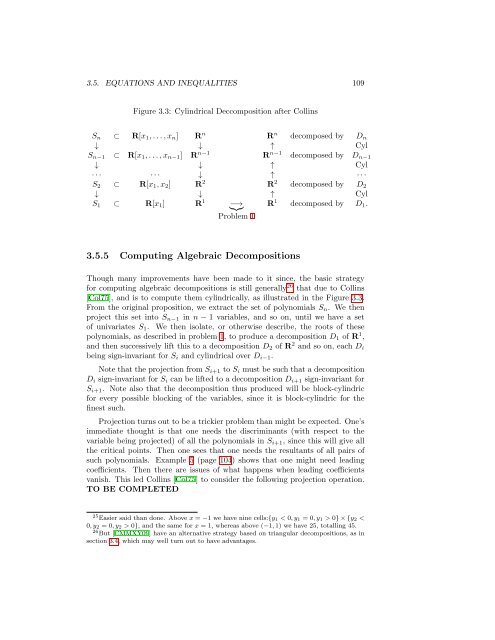
Figure 3.3: Cylindrical Deccomposition after Collins
S n ⊂ R[x 1 , . . . , x n ] R n R n decomposed by D n
↓ ↓ ↑ Cyl
S n−1 ⊂ R[x 1 , . . . , x n−1 ] R n−1 R n−1 decomposed by D n−1
↓ ↓ ↑ Cyl
· · · · · · ↓ ↑ · · ·
S 2 ⊂ R[x 1 , x 2 ] R 2 R 2 decomposed by D 2
↓ ↓ ↑ Cyl
S 1 ⊂ R[x 1 ] R 1 }{{}
−→
Problem 1
R 1 decomposed by D 1 .
3.5.5 Computing Algebraic Decompositions
Though many improvements have been made to it since, the basic strategy
for computing algebraic decompositions is still generally 26 that due to Collins
[Col75], and is to compute them cylindrically, as illustrated in the Figure 3.3.
From the original proposition, we extract the set of polynomials S n . We then
project this set into S n−1 in n − 1 variables, and so on, until we have a set
of univariates S 1 . We then isolate, or otherwise describe, the roots of these
polynomials, as described in problem 1, to produce a decomposition D 1 of R 1 ,
and then successively lift this to a decomposition D 2 of R 2 and so on, each D i
being sign-invariant for S i and cylindrical over D i−1 .
Note that the projection from S i+1 to S i must be such that a decomposition
D i sign-invariant for S i can be lifted to a decomposition D i+1 sign-invariant for
S i+1 . Note also that the decomposition thus produced will be block-cylindric
for every possible blocking of the variables, since it is block-cylindric for the
finest such.
Projection turns out to be a trickier problem than might be expected. One’s
immediate thought is that one needs the discriminants (with respect to the
variable being projected) of all the polynomials in S i+1 , since this will give all
the critical points. Then one sees that one needs the resultants of all pairs of
such polynomials. Example 5 (page 104) shows that one might need leading
coefficients. Then there are issues of what happens when leading coefficients
vanish. This led Collins [Col75] to consider the following projection operation.
TO BE COMPLETED
25 Easier said than done. Above x = −1 we have nine cells:{y 1 < 0, y 1 = 0, y 1 > 0} × {y 2 <
0, y 2 = 0, y 2 > 0}, and the same for x = 1, whereas above (−1, 1) we have 25, totalling 45.
26 But [CMMXY09] have an alternative strategy based on triangular decompositions, as in
section 3.4, which may well turn out to have advantages.