Contents - Student subdomain for University of Bath

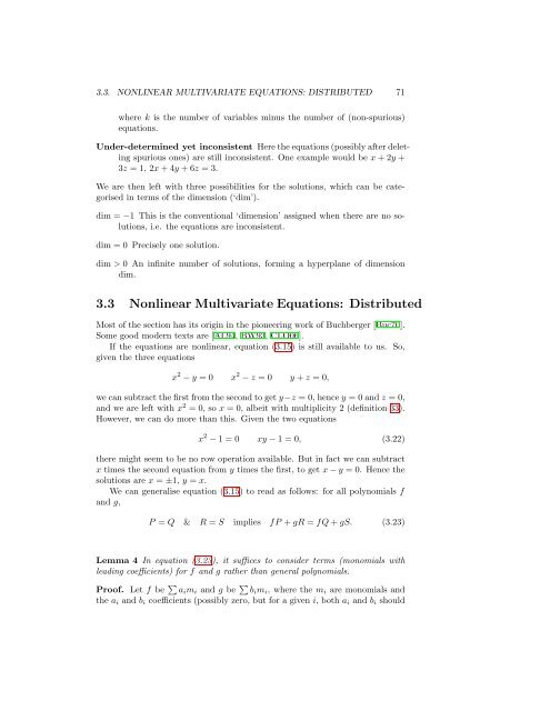
3.3. NONLINEAR MULTIVARIATE EQUATIONS: DISTRIBUTED 71
where k is the number of variables minus the number of (non-spurious)
equations.
Under-determined yet inconsistent Here the equations (possibly after deleting
spurious ones) are still inconsistent. One example would be x + 2y +
3z = 1, 2x + 4y + 6z = 3.
We are then left with three possibilities for the solutions, which can be categorised
in terms of the dimension (‘dim’).
dim = −1 This is the conventional ‘dimension’ assigned when there are no solutions,
i.e. the equations are inconsistent.
dim = 0 Precisely one solution.
dim > 0 An infinite number of solutions, forming a hyperplane of dimension
dim.
3.3 Nonlinear Multivariate Equations: Distributed
Most of the section has its origin in the pioneering work of Buchberger [Buc70].
Some good modern texts are [AL94, BW93, CLO06].
If the equations are nonlinear, equation (3.15) is still available to us. So,
given the three equations
x 2 − y = 0 x 2 − z = 0 y + z = 0,
we can subtract the first from the second to get y−z = 0, hence y = 0 and z = 0,
and we are left with x 2 = 0, so x = 0, albeit with multiplicity 2 (definition 33).
However, we can do more than this. Given the two equations
x 2 − 1 = 0 xy − 1 = 0, (3.22)
there might seem to be no row operation available. But in fact we can subtract
x times the second equation from y times the first, to get x − y = 0. Hence the
solutions are x = ±1, y = x.
We can generalise equation (3.15) to read as follows: for all polynomials f
and g,
P = Q & R = S implies fP + gR = fQ + gS. (3.23)
Lemma 4 In equation (3.23), it suffices to consider terms (monomials with
leading coefficients) for f and g rather than general polynomials.
Proof. Let f be ∑ a i m i and g be ∑ b i m i , where the m i are monomials and
the a i and b i coefficients (possibly zero, but for a given i, both a i and b i should