Contents - Student subdomain for University of Bath

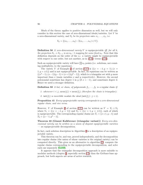
96 CHAPTER 3. POLYNOMIAL EQUATIONS
Much of the theory applies to positive dimension as well, but we will only
consider in this section the case of zero-dimensional ideals/varieties. Let V be
a zero-dimensional variety, and V k be its projection onto x 1 , . . . , x k , i.e.
V k = {(α 1 , . . . , α k ) : ∃(α 1 , . . . , α n ) ∈ V }.
Definition 58 A zero-dimensional variety V is equiprojectable iff, for all k,
the projection V k → V k−1 is an n k : 1 mapping for some fixed n k . Note that this
definition depends on the order of the x i : a variety might be equiprojectable
with respect to one order, but not another, as in (3.32) versus (3.33).
Such an equiprojectable variety will have ∏ n k points (i.e. solutions, not counting
multiplicity, to the equations).
The variety V of Example 2 of section 3.3.7 is {(x = −1, y = 1), (x =
1, y = ±1)} and is not equiprojectable. In fact, its equations can be written as
{(x 2 − 1), (x − 1)(y − 1) + (x + 1)(y 2 − 1)}, which is a triangular set with y more
important than x (main variables x and y respectively). However, the second
polynomial sometimes has degree 1 in y (if x = −1), and sometimes degree 2.
Hence we need a stronger definition.
Definition 59 A list, or chain, of polynomials f 1 , . . . , f k is a regular chain if:
1. whenever i < j, mvar(f i ) ≺ mvar(f j ) (therefore the chain is triangular);
2. init(f i ) is invertible modulo the ideal (init(f j ) : j < i).
Proposition 41 Every equiprojectable variety corresponds to a zero-dimensional
regular chain, and vice versa.
However, V of Example 2 of section 3.3.7 can be written as V = V 1 ∪ V 2
where V 1 = {(x = −1, y = 1)} and V 2 = {(x = 1, y = ±1)}, each of which
is equiprojectable. The corresponding regular chains are T 1 = {x+1, y −1} and
T 2 = {x − 1, y 2 − 1}.
Theorem 22 (Gianni–Kalkbrener (triangular variant)) Every zero-dimensional
variety can be written as a union of disjoint equiprojectable varieties
— an equiprojectable decomposition.
In fact, each solution description in Algorithm 9 is a description of an equiprojectable
variety.
This theorem can be, and was, proved independently, and the decomposition
into regular chains (the union of whose varieties is the original variety) can be
computed directly. This gives us an alternative to algorithm 12: compute the
regular chains corresponding to the equiprojectable decomposition, and solve
each one separately [Laz92].
It appears that the triangular decomposition approach is more suitable to
modular methods (chapter 4, especially section 4.5) than the Gröbner-base approach,
but both aspects are areas of active research.