Contents - Student subdomain for University of Bath

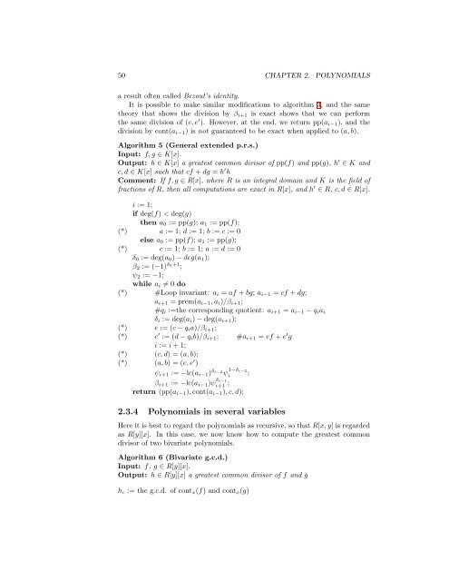
50 CHAPTER 2. POLYNOMIALS
a result often called Bezout’s identity.
It is possible to make similar modifications to algorithm 3, and the same
theory that shows the division by β i+1 is exact shows that we can perform
the same division of (e, e ′ ). However, at the end, we return pp(a i−1 ), and the
division by cont(a i−1 ) is not guaranteed to be exact when applied to (a, b).
Algorithm 5 (General extended p.r.s.)
Input: f, g ∈ K[x].
Output: h ∈ K[x] a greatest common divisor of pp(f) and pp(g), h ′ ∈ K and
c, d ∈ K[x] such that cf + dg = h ′ h
Comment: If f, g ∈ R[x], where R is an integral domain and K is the field of
fractions of R, then all computations are exact in R[x], and h ′ ∈ R, c, d ∈ R[x].
i := 1;
if deg(f) < deg(g)
then a 0 := pp(g); a 1 := pp(f);
(*) a := 1; d := 1; b := c := 0
else a 0 := pp(f); a 1 := pp(g);
(*) c := 1; b := 1; a := d := 0
δ 0 := deg(a 0 ) − deg(a 1 );
β 2 := (−1) δ0+1 ;
ψ 2 := −1;
while a i ≠ 0 do
(*) #Loop invariant: a i = af + bg; a i−1 = cf + dg;
a i+1 = prem(a i−1 , a i )/β i+1 ;
#q i :=the corresponding quotient: a i+1 = a i−1 − q i a i
δ i := deg(a i ) − deg(a i+1 );
(*) e := (c − q i a)/β i+1 ;
(*) e ′ := (d − q i b)/β i+1 ; #a i+1 = ef + e ′ g
i := i + 1;
(*) (c, d) = (a, b);
(*) (a, b) = (e, e ′ )
ψ i+1 := −lc(a i−1 ) δi−2 ψ 1−δi−2
i ;
i+1 ;
β i+1 := −lc(a i−1 )ψ δi−1
return (pp(a i−1 ), cont(a i−1 ), c, d);
2.3.4 Polynomials in several variables
Here it is best to regard the polynomials as recursive, so that R[x, y] is regarded
as R[y][x]. In this case, we now know how to compute the greatest common
divisor of two bivariate polynomials.
Algorithm 6 (Bivariate g.c.d.)
Input: f, g ∈ R[y][x].
Output: h ∈ R[y][x] a greatest common divisor of f and g
h c := the g.c.d. of cont x (f) and cont x (g)