Contents - Student subdomain for University of Bath

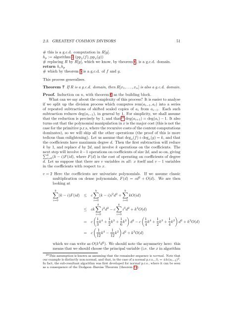
2.3. GREATEST COMMON DIVISORS 51
# this is a g.c.d. computation in R[y].
h p := algorithm 3 (pp x (f), pp x (g))
# replacing R by R[y], which we know, by theorem 6, is a g.c.d. domain.
return h c h p
# which by theorem 5 is a g.c.d. of f and g.
This process generalises.
Theorem 7 If R is a g.c.d. domain, then R[x 1 , . . . , x n ] is also a g.c.d. domain.
Proof. Induction on n, with theorem 6 as the building block.
What can we say about the complexity of this process? It is easier to analyse
if we split up the division process which computes rem(a i−1 , a i ) into a series
of repeated subtractions of shifted scaled copies of a i from a i−1 . Each such
subtraction reduces deg(a i−1 ), in general by 1. For simplicity, we shall assume
that the reduction is precisely by 1, and that 28 deg(a i+1 ) = deg(a i ) − 1. It also
turns out that the polynomial manipulation in x is the major cost (this is not the
case for the primitive p.r.s, where the recursive costs of the content computations
dominates), so we will skip all the other operations (the proof of this is more
tedious than enlightening). Let us assume that deg x (f)+deg x (g) = k, and that
the coefficients have maximum degree d. Then the first subtraction will reduce
k by 1, and replace d by 2d, and involve k operations on the coefficients. The
∑
next step will involve k−1 operations on coefficients of size 2d, and so on, giving
k
i=0
(k − i)F (id), where F (d) is the cost of operating on coefficients of degree
d. Let us suppose that there are v variables in all: x itself and v − 1 variables
in the coefficients with respect to x.
v = 2 Here the coefficients are univariate polynomials. If we assume classic
multiplication on dense polynomials, F (d) = cd 2 + O(d). We are then
looking at
k∑
(k − i)F (id) ≤ c
i=0
≤
ck
k∑
(k − i)i 2 d 2 +
i=0
k∑
i 2 d 2 − c
i=0
k∑
kO(id)
i=0
k∑
i 3 d 2 + k 3 O(d)
i=0
( 1
= c
3 k4 + 1 2 k3 + 1 ) ( 1
6 k2 d 2 − c
4 k4 + 1 2 k3 + 1 )
4 k2 d 2 + k 3 O(d)
( 1
= c
12 k4 − 1 )
12 k2 d 2 + k 3 O(d)
which we can write as O(k 4 d 2 ). We should note the asymmetry here: this
means that we should choose the principal variable (i.e. the x in algorithm
28 This assumption is known as assuming that the remainder sequence is normal. Note that
our example is distinctly non-normal, and that, in the case of a normal p.r.s., β i = ±lc(a i−2 ) 2 .
In fact, the sub-resultant algorithm was first developed for normal p.r.s., where it can be seen
as a consequence of the Dodgson–Bareiss Theorem (theorem 12).