Contents - Student subdomain for University of Bath

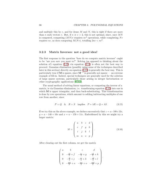
66 CHAPTER 3. POLYNOMIAL EQUATIONS
and multiply this by v, and for dense M and N, this is right if there are more
than n such vectors v. But, if n ≫ e > 2, this is not optimal, since, once MN
is computed, computing (MN)v requires ne 2 operations, while compluting Nv
requires ne, as does computing M(Nv), totalling 2ne < ne 2 .
3.2.3 Matrix Inverses: not a good idea!
The first response to the question “how do we compute matrix inverses” ought
to be “are you sure you want to?” Solving (as opposed to thinking about the
solution of) equation (3.13) via equation (3.14) is often not the best way to
proceed. Gaussian elimination (possibly using some of the techniques described
later in this section) directly on equation (3.13) is generally the best way. This is
particularly true if M is sparse, since M −1 is generally not sparse — an extreme
example of fill-in. Indeed, special techniques are generally used for the solution
of large sparse systems, particularly those arising in integer factorisation or
other cryptographic applications [HD03].
The usual method of solving linear equations, or computing the inverse of a
matrix, is via Gaussian elimination, i.e. transforming equation (3.13) into one in
which M is upper triangular, and then back-substituting. This transformation
is done by row operations, which amount to adding/subtracting multiples of one
row from another, since
P = Q & R = S implies P + λR = Q + λS. (3.15)
If we try this on the above example, we deduce successively that z = a−18b+13c,
y = a − 14b + 10c and x = a − 15b + 11c. Emboldened by this we might try a
larger matrix:
⎛
⎞
a b c d
e f g h
M =
. (3.16)
⎜
⎝
i j k l ⎟
⎠
m n o p
After clearing out the first column, we get the matrix
⎛
⎜
⎝
⎞
a b c d
0 − eb
a + f − ec
a + g − ed a + h
0 − ib a + j − ic a + k − id a + l
.
⎟
⎠
0 − mb
a + n − mc
a + o − md
a
+ p