Observational Constraints on The Evolution of Dust in ...
Observational Constraints on The Evolution of Dust in ...
Observational Constraints on The Evolution of Dust in ...

You also want an ePaper? Increase the reach of your titles
YUMPU automatically turns print PDFs into web optimized ePapers that Google loves.
56 YSOs <strong>in</strong> the Lupus Molecular Clouds<br />
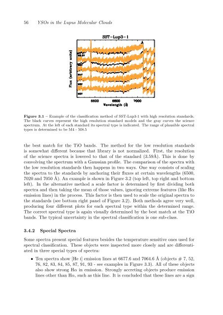
Figure 3.1 – Example <strong>of</strong> the classificati<strong>on</strong> method <strong>of</strong> SST-Lup3-1 with high resoluti<strong>on</strong> standards.<br />
<strong>The</strong> black curves represent the high resoluti<strong>on</strong> standard models and the gray curves the science<br />
spectrum. At the left <strong>of</strong> each standard its spectral type is <strong>in</strong>dicated. <strong>The</strong> range <strong>of</strong> plausible spectral<br />
types is determ<strong>in</strong>ed to be M4 - M8.5<br />
the best match for the TiO bands. <strong>The</strong> method for the low resoluti<strong>on</strong> standards<br />
is somewhat different because that library is not normalized. First, the resoluti<strong>on</strong><br />
<strong>of</strong> the science spectra is lowered to that <strong>of</strong> the standard (3.59Å). This is d<strong>on</strong>e by<br />
c<strong>on</strong>volv<strong>in</strong>g the spectrum with a Gaussian pr<strong>of</strong>ile. <strong>The</strong> comparis<strong>on</strong> <strong>of</strong> the spectra with<br />
the low resoluti<strong>on</strong> standards then happens <strong>in</strong> two ways. One way c<strong>on</strong>sists <strong>of</strong> scal<strong>in</strong>g<br />
the spectra to the standards by anchor<strong>in</strong>g their fluxes at certa<strong>in</strong> wavelengths (6500,<br />
7020 and 7050 Å). An example is shown <strong>in</strong> Figure 3.2 (top left, top right and bottom<br />
left). In the alternative method a scale factor is determ<strong>in</strong>ed by first divid<strong>in</strong>g both<br />
spectra and then tak<strong>in</strong>g the mean <strong>of</strong> those values, ignor<strong>in</strong>g extreme features (like Hα<br />
emissi<strong>on</strong> l<strong>in</strong>es) <strong>in</strong> the process. This factor is then used to scale the orig<strong>in</strong>al spectra to<br />
the standards (see bottom right panel <strong>of</strong> Figure 3.2). Both methods agree very well,<br />
produc<strong>in</strong>g four different plots for each spectral type with<strong>in</strong> the determ<strong>in</strong>ed range.<br />
<strong>The</strong> correct spectral type is aga<strong>in</strong> visually determ<strong>in</strong>ed by the best match at the TiO<br />
bands. <strong>The</strong> typical uncerta<strong>in</strong>ty <strong>in</strong> the spectral classificati<strong>on</strong> is <strong>on</strong>e sub-class.<br />
3.4.2 Special Spectra<br />
Some spectra present special features besides the temperature sensitive <strong>on</strong>es used for<br />
spectral classificati<strong>on</strong>. <strong>The</strong>se objects were <strong>in</strong>spected more closely and are differentiated<br />
<strong>in</strong> three special types <strong>of</strong> spectra:<br />
• Ten spectra show [He i] emissi<strong>on</strong> l<strong>in</strong>es at 6677.6 and 7064.6 Å (objects # 7, 52,<br />
76, 82, 83, 84, 85, 87, 91, 93 - see examples <strong>in</strong> Figure 3.3). All <strong>of</strong> these objects<br />
also show str<strong>on</strong>g Hα <strong>in</strong> emissi<strong>on</strong>. Str<strong>on</strong>gly accret<strong>in</strong>g objects produce emissi<strong>on</strong><br />
l<strong>in</strong>es other than Hα, such as this l<strong>in</strong>e. It is c<strong>on</strong>cluded that these l<strong>in</strong>es are a sign