Session B.pdf - Clarkson University

heat exchange simulation on the boundary of the water surface with the atmosphere taking
into account the possibility of ice formation and melting. At that this task has to be
solved namely at unsteady setting taking into account the dynamics of weather factors
changing: air temperature, wind velocity and direction, air humidity, precipitation intensity,
cloudiness and so on. Unsteadiness imposes strict demands on the efficiency of the
used numerical method especially if the task is solved in three-dimensional (3D) setting.
There is a number of different approaches to solve the task with the majority of which
are based on one-dimensional [1] or plane (2D) [2-4] setting.
2D and 3D algorithms given in this work are made up on the method of the finite volume
that allows to create numerical diagrams conservative by mass and pulse [5-7]. For
the tasks connected with unsteady heat transmission the conservatism of the numerical
diagram is an obligatory condition.
Plane (2D) Model of Hydro-Dynamics and Heat Transmission
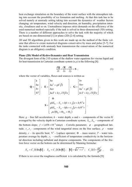
The divergent form of the 2-D system of the shallow water equations for viscous liquid and
for heat transmission in Cartesian coordinate system (x,y) is the following [8]:
where the vector of variables, fluxes and sources is written as
∂Q
∂E
∂G
+ + = S , (1)
∂t
∂x
∂y
⎡h
⎤ ⎡hu
⎤ ⎡hv
⎢ ⎢ 2 2 ⎥ ⎢
hu
⎥
⎢ ⎥
2
; ⎢
hu + gh
huv
Q = E =
⎥ ; G = ⎢
2 2
⎢hv
⎥ ⎢huv
⎥ ⎢hu
+ gh 2
⎢ ⎥ ⎢
⎥ ⎢
⎣hT
⎦ ⎣huT
+ hγ T
∂T
∂x⎦
⎣hvT
+ hγ T
∂T
⎡ Φ
⎤
⎢
2
⎢
ghS0x
− S
fx
+ hfv + τ
x
ρ + hγ∇
u
S =
.
⎢
2
ghS0
y
− S
fy
− hfu + τ
y
ρ + hγ∇
v
⎢
⎢⎣
ρc
( ) ⎥ ⎥⎥⎥⎥ ΘΦ
+ Θbot
+ ΘS
⎦
⎤
⎥
⎥
⎥
⎥
∂y⎦
Here: g – free fall acceleration; h – water depth; u and v – components of the vector U
averaged by the velocity depth in Cartesian coordinate system; S – components of
S0 x,
0 y
−4
the bottom slope; f = 1,458 × 10 sin( ϕ)
– Coriolis parameter, ϕ – geographical latitude;
τ
x
, τ
y
– components of the wind tangential stress on the free surface; ρ – water
2
density, c – its specific heat; ∇ – Laplace operator; Φ – mass source; T – water temperature
average by depth; γ
T
– coefficient of temperature conductivity in the horizontal
direction including turbulent and disperse components. The components of the friction
force vector on the bottom can be determined by Manning formulae:
S
2
2 2
gn
= C
f
( h) hu U ; S
fy
= C
f
( h) hv U ; U = u + v ; C
f
( h) . (2)
4 3
h
fx
=
If there is ice cover the roughness coefficient n is calculated by the formula [9]:
;
160