Session B.pdf - Clarkson University

k k
( sL
, sR
) max( γ , γ )
4
⎪
⎧
1 ⎡max
⎤⎪
⎫
k
T
∆t
< Cr max⎨
∑ A ⎢
+ ⎥⎬
, (11)
i,
j Ω k = 1 2 ( )
⎪⎩ ⎢
n ⋅
⎣
k
rk
⎥⎦
⎪⎭
where r k
– the vector from the center of the finite volume up to the nearby (through the
k edge) node; sL, s R – wave numbers at the left and at the right of the FV bound [13,15].
The Curant number Cr for all carried out calculations was chosen in the interval of 0,7-
0,95.
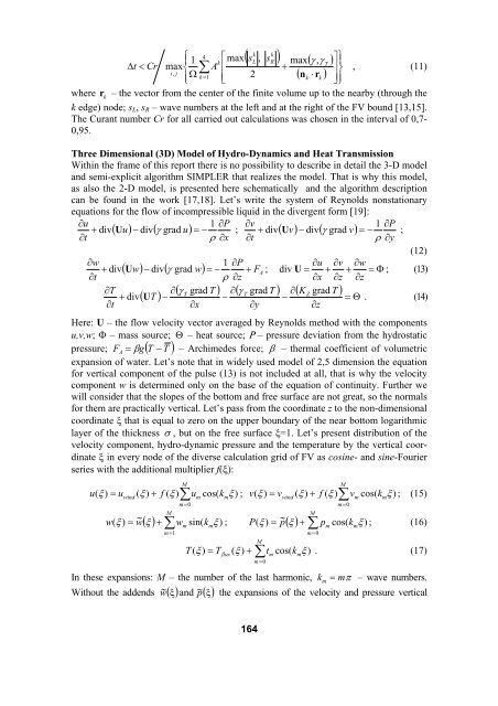
Three Dimensional (3D) Model of Hydro-Dynamics and Heat Transmission
Within the frame of this report there is no possibility to describe in detail the 3-D model
and semi-explicit algorithm SIMPLER that realizes the model. That is why this model,
as also the 2-D model, is presented here schematically and the algorithm description
can be found in the work [17,18]. Let’s write the system of Reynolds nonstationary
equations for the flow of incompressible liquid in the divergent form [19]:
∂u
1 ∂P
∂v
1 ∂P
+ div( U u) − div( γ grad u)
= − ; + div( U v) − div( γ grad v)
= − ;
∂t
ρ ∂x
∂t
ρ ∂y
(12)
∂w
1 ∂P
∂u
∂v
∂w
+ div( U w) − div( γ grad w) = − + FA
; div U = + + = Φ ; (13)
∂t
ρ ∂z
∂x
∂z
∂z
∂T
∂
( )
( γ
T
grad T ) ∂( γ
T
grad T ) ∂( KZ
grad T )
+ div U T −
−
−
= Θ . (14)
∂t
∂x
∂y
∂z
Here: U – the flow velocity vector averaged by Reynolds method with the components
u,v,w; Φ – mass source; Θ – heat source; Ρ – pressure deviation from the hydrostatic
pressure; F A
= β g( T − T ) – Archimedes force; β – thermal coefficient of volumetric
expansion of water. Let’s note that in widely used model of 2,5 dimension the equation
for vertical component of the pulse (13) is not included at all, that is why the velocity
component w is determined only on the base of the equation of continuity. Further we
will consider that the slopes of the bottom and free surface are not great, so the normals
for them are practically vertical. Let’s pass from the coordinate z to the non-dimensional
coordinate ξ that is equal to zero on the upper boundary of the near bottom logarithmic
layer of the thickness σ , but on the free surface ξ=1. Let’s present distribution of the
velocity component, hydro-dynamic pressure and the temperature by the vertical coordinate
ξ in every node of the diverse calculation grid of FV as cosine- and sine-Fourier
series with the additional multiplier f(ξ):
M
u(
ξ ) = u ( ξ ) + f ( ξ ) u cos( k ξ ) ; v(
ξ ) = v ( ξ ) + f ( ξ ) v cos( k ξ ) ; (15)
wind
M
∑
m=
0
m
( ξ ) + w m
sin( k ξ )
m
wind
M
∑
m
m=
0
w(
ξ ) = w~
; P(
ξ ) = ~ p ξ + p m
cos( k ξ ; (16)
∑
m=
1
m
M
M
( ) )
∑
m=
0
T ( ξ ) = T ( ξ ) + t cos( k ξ ) . (17)
flux
∑
m
m=
0
In these expansions: M – the number of the last harmonic, k m
= mπ
– wave numbers.
w ~ ξ and ~ p ξ the expansions of the velocity and pressure vertical
Without the addends ( ) ( )
m
m
m
164