Session B.pdf - Clarkson University

increasingly necessary in the future. Because hardly any field observations are available
in Okhotsk Sea coast of Hokkaido, we have conducted sea ice surveys using IPS (Ice
Profiling Sonar) since 2000. In 2001, ADCP (Acoustic Doppler Current Profiler) was
added to the survey to focus primarily on drift characteristics of pack ice and to provide a
means to change the temporal IPS data set to spatial data set. Theories and survey
methods of these measuring instruments were detailed by Sakikawa et al. (2002), Belliveau
et al. (1989) and Birch et al. (1999). Some of the survey results including the
characteristics of sea ice drift have already been reported (Sakikawa et al., 2002; Yamamoto
et al., 2002, Yamamoto et al., 2003). Furthermore, sea ice surveys using the same
measuring instruments (IPS and ADCP) have been conducted in the northeastern part of
Sakhalin (Birch et al.; 1999).
This study quantitatively analyzed the bottom unevenness (roughness) or draft profile of
sea ice using spectrum analysis (locally stationary AR model) and time-frequency
analysis (Discrete Wavelet Transformation). We examined methods for representing
typical unevenness characteristics of the sea ice bottom, methods that can produce input
for simulation of ice draft profile or the bottom unevenness.
SURVEY AND ICE DRAFT PROFILE [Yamamoto et al., 2002]
The observation site was 2.4 km off the coast of Mombetsu, Hokkaido. An Acoustic
Doppler Current Profiler (ADCP) and an Ice Profiling Sonar (IPS) were installed at a
depth of 18 m for continuous observation of the draft and drift speed/direction of sea ice
passing over the observation equipment. Detailed observation methods were described by
Sakikawa et al. (2002) and Yamamoto et al. -20 0 20 40 60 80 (km)
(2002).
20
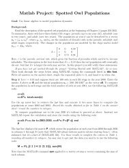
Figure 1 shows a nominal locus of sea ice drift
between February 8 and 19, 2001, when sea ice
existed. Note that this figure constitutes a simple
coordinate based on sea ice drift direction and
velocity data at one fixed location, instead of an
essential locus of sea ice motion [Yamamoto et
al., 2002]. Sea ice mainly moved southward
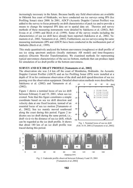
along the coast during this period. Figure 2 indicates
sea ice draft during the same period, i.e.,
draft vis-à-vis the distance of sea ice drift, which
can be regarded as the ice draft profile. It shows
that about 180 km of an ice draft profile was
traced during this period.
0
-20
-40
-60
-80
-100
A
A 2/8 14:00 - 2/9 6:00
B 2/12 8:40 - 2/12 12:00
C 2/19 6:30 - 2/19 10:50
AE 2/15 3:30 - 2/15 9:20
BE 2/18 6:00 - 2/18 8:20
B
EA
EB
Fig. 1. Nominal locus of sea ice drift
(Feb. 8-19, 2001) [Yamamoto et al.,2002]
C
A
B
AE
BE
C
Fig. 2. Underside profile observed between February 8 and 19, 2001
[Yamamoto.et al.,2002]
192