Session B.pdf - Clarkson University

ithm is derived from the two-scale relationships that satisfy the scaling function. Using
this algorithm, Equation (2) is sequentially calculated according to j, which denotes the
level of decomposition.
The 4th order B-spline is chosen as the scaling function, from which the mother wavelet
can be derived (Figure 4).
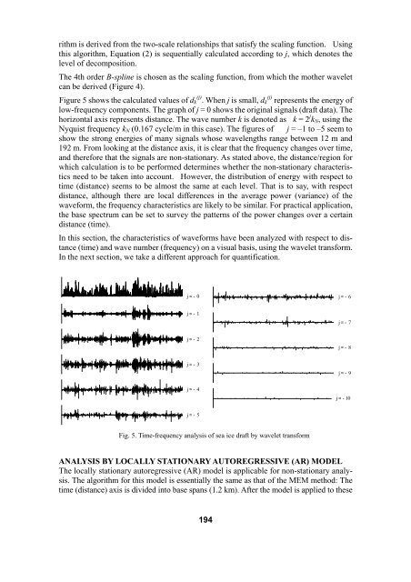
Figure 5 shows the calculated values of d (j) k . When j is small, d (j) k represents the energy of
low-frequency components. The graph of j = 0 shows the original signals (draft data). The
horizontal axis represents distance. The wave number k is denoted as k = 2 j k N , using the
Nyquist frequency k N (0.167 cycle/m in this case). The figures of j = –1 to –5 seem to
show the strong energies of many signals whose wavelengths range between 12 m and
192 m. From looking at the distance axis, it is clear that the frequency changes over time,
and therefore that the signals are non-stationary. As stated above, the distance/region for
which calculation is to be performed determines whether the non-stationary characteristics
need to be taken into account. However, the distribution of energy with respect to
time (distance) seems to be almost the same at each level. That is to say, with respect
distance, although there are local differences in the average power (variance) of the
waveform, the frequency characteristics are likely to be similar. For practical application,
the base spectrum can be set to survey the patterns of the power changes over a certain
distance (time).
In this section, the characteristics of waveforms have been analyzed with respect to distance
(time) and wave number (frequency) on a visual basis, using the wavelet transform.
In the next section, we take a different approach for quantification.
j =-0
j =-6
j =-1
j =-7
j =-2
j =-8
j =-3
j =-9
j =-4
j =-10
j =-5
Fig. 5. Time-frequency analysis of sea ice draft by wavelet transform
ANALYSIS BY LOCALLY STATIONARY AUTOREGRESSIVE (AR) MODEL
The locally stationary autoregressive (AR) model is applicable for non-stationary analysis.
The algorithm for this model is essentially the same as that of the MEM method: The
time (distance) axis is divided into base spans (1.2 km). After the model is applied to these
194