Chapter 4: Programming in Matlab - College of the Redwoods
Chapter 4: Programming in Matlab - College of the Redwoods
Chapter 4: Programming in Matlab - College of the Redwoods

You also want an ePaper? Increase the reach of your titles
YUMPU automatically turns print PDFs into web optimized ePapers that Google loves.
Section 4.1 Logical Arrays 287<br />
prime between 100 and 1000.<br />
In Exercises 23-26, perform each <strong>of</strong><br />
<strong>the</strong> follow<strong>in</strong>g tasks for <strong>the</strong> given function.<br />
i. Write an “array smart” anonymous<br />
function f for <strong>the</strong> given function.<br />
Test your anonymous function before<br />
proceed<strong>in</strong>g.<br />
ii. Set x=l<strong>in</strong>space(-10,10,200) and<br />
evaluate <strong>the</strong> function with y=f(x).<br />
iii. Use <strong>the</strong> plot(x,y) command to plot<br />
<strong>the</strong> function.<br />
iv. Use axis([-10,10,-10,10]) to set<br />
<strong>the</strong> w<strong>in</strong>dow boundaries.<br />
v. Use logical <strong>in</strong>dex<strong>in</strong>g to set all <strong>of</strong><br />
<strong>the</strong> complex entries <strong>in</strong> <strong>the</strong> vector<br />
y to NaN. Open a second figure<br />
w<strong>in</strong>dow with <strong>the</strong> command figure.<br />
Replot <strong>the</strong> result and reset <strong>the</strong> w<strong>in</strong>dow<br />
boundaries as above, if necessary.<br />
Add axis labels and a title<br />
and turn <strong>the</strong> grid on.<br />
23. f(x) = 2 + √ x + 5<br />
24. f(x) = 3 − √ x − 3<br />
25. f(x) = √ 9 − x 2<br />
26. f(x) = √ x 2 − 25<br />
In Exercises 27-30, use “advanced<br />
plann<strong>in</strong>g” to plot <strong>the</strong> given function<br />
on a subset <strong>of</strong> <strong>the</strong> doma<strong>in</strong> [−10, 10]<br />
to avoid complex entries when evaluat<strong>in</strong>g<br />
<strong>the</strong> given function. In each<br />
case, set <strong>the</strong> w<strong>in</strong>dow boundaries with<br />
<strong>the</strong> command axis([-10,10,-10,10]),<br />
turn on <strong>the</strong> grid, and add axes labels<br />
and a title.<br />
27. The function <strong>in</strong> Exercise 23.<br />
28. The function <strong>in</strong> Exercise 24.<br />
29. The function <strong>in</strong> Exercise 25.<br />
30. The function <strong>in</strong> Exercise 26.<br />
In Exercises 31-34, perform each <strong>of</strong><br />
<strong>the</strong> follow<strong>in</strong>g tasks for <strong>the</strong> given function.<br />
i. Write an “array smart” anonymous<br />
function f for <strong>the</strong> given function.<br />
Test your anonymous function before<br />
proceed<strong>in</strong>g.<br />
ii. Set:<br />
x=l<strong>in</strong>space(-3,3,40);<br />
y=x;<br />
[x,y]=meshgrid(x,y);<br />
Evaluate <strong>the</strong> function with z=f(x,y).<br />
iii. Use mesh(x,y,z) to plot <strong>the</strong> surface<br />
def<strong>in</strong>ed by <strong>the</strong> function.<br />
iv. Use logical <strong>in</strong>dex<strong>in</strong>g to set all <strong>of</strong><br />
<strong>the</strong> complex entries <strong>in</strong> <strong>the</strong> vector<br />
z to NaN. Open a second figure<br />
w<strong>in</strong>dow with <strong>the</strong> command figure.<br />
Replot <strong>the</strong> surface. Add axis labels<br />
and a title.<br />
31. f(x, y) = √ 1 + x<br />
32. f(x, y) = √ 1 − y<br />
33. f(x, y) = √ 9 − x 2 − y 2<br />
34. f(x, y) = √ x 2 + y 2 − 1<br />
In Exercises 35-40, perform each <strong>of</strong><br />
<strong>the</strong> follow<strong>in</strong>g tasks for <strong>the</strong> given func-