Chapter 4: Programming in Matlab - College of the Redwoods
Chapter 4: Programming in Matlab - College of the Redwoods
Chapter 4: Programming in Matlab - College of the Redwoods

You also want an ePaper? Increase the reach of your titles
YUMPU automatically turns print PDFs into web optimized ePapers that Google loves.
Section 4.2 Control Structures <strong>in</strong> <strong>Matlab</strong> 319<br />
(a)<br />
Figure 4.7.<br />
(b)<br />
Generat<strong>in</strong>g a square wave with mod.<br />
Let’s make one last adjustment, <strong>in</strong>creas<strong>in</strong>g <strong>the</strong> amplitude by 2, <strong>the</strong>n shift<strong>in</strong>g <strong>the</strong><br />
graph downward 1 unit. This produces <strong>the</strong> square wave shown <strong>in</strong> Figure 4.8.<br />
y=2*y-1;<br />
plot(t,y,’*’)<br />
Figure 4.8. A square<br />
wave with period 2.<br />
Note that this square waves alternates between <strong>the</strong> values 1 and −1. The curve<br />
equals 1 on <strong>the</strong> first half <strong>of</strong> its period, <strong>the</strong>n −1 on its second half. This pattern<br />
<strong>the</strong>n repeats with period 2 over <strong>the</strong> rema<strong>in</strong>der <strong>of</strong> its doma<strong>in</strong>.<br />
Fourier Series. Us<strong>in</strong>g advanced ma<strong>the</strong>matics, it can be shown that <strong>the</strong><br />
follow<strong>in</strong>g Fourier Series “converges” to <strong>the</strong> square wave pictured <strong>in</strong> Figure 4.8<br />
∞∑ 4<br />
s<strong>in</strong>(2n + 1)πt (4.4)<br />
(2n + 1)π<br />
n=0