Chapter 4: Programming in Matlab - College of the Redwoods
Chapter 4: Programming in Matlab - College of the Redwoods
Chapter 4: Programming in Matlab - College of the Redwoods

Create successful ePaper yourself
Turn your PDF publications into a flip-book with our unique Google optimized e-Paper software.
Section 4.2 Control Structures <strong>in</strong> <strong>Matlab</strong> 321<br />
However, a truly remarkable result occurs when we add <strong>the</strong> s<strong>in</strong>usoids <strong>in</strong><br />
Figure 4.9(a). This is easy to do because we saved each <strong>in</strong>dividual term <strong>in</strong><br />
a row <strong>of</strong> matrix A. <strong>Matlab</strong>’s sum command will sum <strong>the</strong> columns <strong>of</strong> matrix A,<br />
effectively summ<strong>in</strong>g <strong>the</strong> first five terms <strong>of</strong> series (4.4) at each <strong>in</strong>stant <strong>of</strong> time t.<br />
figure<br />
plot(t,sum(A))<br />
We “tighten” <strong>the</strong> axes, add a grid, <strong>the</strong>n annotate each axis. This produces<br />
<strong>the</strong> image <strong>in</strong> Figure 4.9(b). Note <strong>the</strong> strik<strong>in</strong>g similarity to <strong>the</strong> square wave<br />
<strong>in</strong> Figure 4.8.<br />
axis tight<br />
grid on<br />
xlabel(’t-axis’)<br />
ylabel(’y-axis’)<br />
Figure 4.9.<br />
(a)<br />
Approximat<strong>in</strong>g a square wave with a Fourier series (5 terms).<br />
(b)<br />
Because we smartly stored <strong>the</strong> number <strong>of</strong> terms <strong>in</strong> <strong>the</strong> variable numterms,<br />
to see <strong>the</strong> effect <strong>of</strong> add<strong>in</strong>g <strong>the</strong> first 10 terms <strong>of</strong> <strong>the</strong> fourier series (4.4) is a simple<br />
matter <strong>of</strong> chang<strong>in</strong>g numterms=5 to numterms=10 and runn<strong>in</strong>g <strong>the</strong> program<br />
aga<strong>in</strong>. The ouptut is shown <strong>in</strong> Figures 4.10(a) and (b). In Figure 4.10(b),<br />
note <strong>the</strong> even closer resemblance to <strong>the</strong> square wave <strong>in</strong> Figure 4.8, except at <strong>the</strong><br />
ends, where <strong>the</strong> “r<strong>in</strong>g<strong>in</strong>g” exhibited <strong>the</strong>re is known as Gibb’s Phenomenon. If you