Intel® Trace Analyzer User's Reference Guide
Intel® Trace Analyzer User's Reference Guide
Intel® Trace Analyzer User's Reference Guide

Create successful ePaper yourself
Turn your PDF publications into a flip-book with our unique Google optimized e-Paper software.
Intel® <strong>Trace</strong> <strong>Analyzer</strong><br />
<strong>User's</strong> <strong>Reference</strong> <strong>Guide</strong>
Intel® <strong>Trace</strong> <strong>Analyzer</strong> <strong>User's</strong> <strong>Reference</strong> <strong>Guide</strong><br />
Intel® <strong>Trace</strong> <strong>Analyzer</strong> <strong>User's</strong> <strong>Reference</strong> <strong>Guide</strong><br />
Disclaimer and Legal Information<br />
The information in this manual is subject to change without notice and Intel Corporation assumes no responsibility<br />
or liability for any errors or inaccuracies that may appear in this document or any software that may be provided<br />
in association with this document. This document and the software described in it are furnished under license and<br />
may only be used or copied in accordance with the terms of the license. No license, express or implied, by estoppel<br />
or otherwise, to any intellectual property rights is granted by this document. The information in this document is<br />
provided in connection with Intel products and should not be construed as a commitment by Intel Corporation.<br />
INFORMATION IN THIS DOCUMENT IS PROVIDED IN CONNECTION WITH INTEL(R) PRODUCTS. NO LICENSE,<br />
EXPRESS OR IMPLIED, BY ESTOPPEL OR OTHERWISE, TO ANY INTELLECTUAL PROPERTY RIGHTS IS GRANTED BY<br />
THIS DOCUMENT. EXCEPT AS PROVIDED IN INTEL'S TERMS AND CONDITIONS OF SALE FOR SUCH PRODUCTS,<br />
INTEL ASSUMES NO LIABILITY WHATSOEVER, AND INTEL DISCLAIMS ANY EXPRESS OR IMPLIED WARRANTY,<br />
RELATING TO SALE AND/OR USE OF INTEL PRODUCTS INCLUDING LIABILITY OR WARRANTIES RELATING TO<br />
FITNESS FOR A PARTICULAR PURPOSE, MERCHANTABILITY, OR INFRINGEMENT OF ANY PATENT, COPYRIGHT OR<br />
OTHER INTELLECTUAL PROPERTY RIGHT.<br />
UNLESS OTHERWISE AGREED IN WRITING BY INTEL, THE INTEL PRODUCTS ARE NOT DESIGNED NOR INTENDED<br />
FOR ANY APPLICATION IN WHICH THE FAILURE OF THE INTEL PRODUCT COULD CREATE A SITUATION WHERE<br />
PERSONAL INJURY OR DEATH MAY OCCUR.<br />
Intel may make changes to specifications and product descriptions at any time, without notice. Designers must<br />
not rely on the absence or characteristics of any features or instructions marked "reserved" or "undefined." Intel<br />
reserves these for future definition and shall have no responsibility whatsoever for conflicts or incompatibilities<br />
arising from future changes to them. The information here is subject to change without notice. Do not finalize<br />
a design with this information.<br />
The products described in this document may contain design defects or errors known as errata which may cause<br />
the product to deviate from published specifications. Current characterized errata are available on request.<br />
Contact your local Intel sales office or your distributor to obtain the latest specifications and before placing your<br />
product order.<br />
Copies of documents which have an order number and are referenced in this document, or other Intel literature,<br />
may be obtained by calling 1-800-548-4725, or by visiting http://www.intel.com.<br />
Intel, Itanium, Pentium, VTune, and Xeon are trademarks of Intel Corporation in the U.S. and other countries.<br />
* Other names and brands may be claimed as the property of others.<br />
Copyright (c) 1996-2009, Intel Corporation. All rights reserved.<br />
Intel® <strong>Trace</strong> <strong>Analyzer</strong> ships libraries licensed under the GNU Lesser Public License (LGPL) or Runtime General<br />
Public License. Their source code can be downloaded from ftp://ftp.ikn.intel.com/pub/opensource.<br />
Document number: 318120-002 2
Intel® <strong>Trace</strong> <strong>Analyzer</strong> <strong>User's</strong> <strong>Reference</strong> <strong>Guide</strong><br />
Document number: 318120-002 3
Intel® <strong>Trace</strong> <strong>Analyzer</strong> <strong>User's</strong> <strong>Reference</strong> <strong>Guide</strong><br />
Table of Contents<br />
1. Introduction ..................................................................................... 1<br />
Notation and Terms ........................................................................ 1<br />
Starting the Intel® <strong>Trace</strong> <strong>Analyzer</strong> ................................................... 1<br />
Starting in a UNIX* Environment ............................................... 1<br />
Starting in a Windows* Environment .......................................... 2<br />
The <strong>Trace</strong> Cache ...................................................................... 2<br />
The Command Line Interface (CLI) ............................................ 2<br />
Internationalization ......................................................................... 2<br />
Online Resources ........................................................................... 4<br />
For the Impatient ........................................................................... 4<br />
2. The Main Menu ............................................................................... 10<br />
The File Menu .............................................................................. 10<br />
The Style Menu ............................................................................ 10<br />
The Windows Menu ...................................................................... 11<br />
The Help Menu ............................................................................ 12<br />
3. Views ............................................................................................ 13<br />
The View's Main Menu .................................................................. 13<br />
The View Menu ..................................................................... 13<br />
The Charts Menu ................................................................... 14<br />
The Navigate Menu ................................................................ 15<br />
The Advanced Menu ............................................................... 17<br />
The Layout Menu ................................................................... 18<br />
The Comparison Menu ............................................................ 20<br />
The Status Bar ............................................................................ 20<br />
Navigation In Time ....................................................................... 21<br />
The Zoom Stack .................................................................... 21<br />
4. Charts ........................................................................................... 24<br />
Event Timeline ............................................................................. 24<br />
Mouse Hover ......................................................................... 25<br />
Event Timeline Settings .......................................................... 25<br />
The Context Menu ................................................................. 27<br />
Filtering and Tagging .............................................................. 28<br />
Qualitative Timeline ...................................................................... 28<br />
Mouse Hover ......................................................................... 29<br />
Qualitative Timeline Settings ................................................... 30<br />
Context Menu ........................................................................ 31<br />
Filtering and Tagging .............................................................. 31<br />
Quantitative Timeline .................................................................... 32<br />
Mouse Hover ......................................................................... 32<br />
Quantitative Timeline Settings ................................................. 33<br />
The Context Menu ................................................................. 34<br />
Filtering and Tagging .............................................................. 35<br />
Counter Timeline .......................................................................... 36<br />
Mouse Hover ......................................................................... 37<br />
Counter Timeline Settings ....................................................... 37<br />
The Context Menu ................................................................. 39<br />
Filtering and Tagging .............................................................. 39<br />
The Function Profile Chart ............................................................. 39<br />
Flat Profile ............................................................................ 40<br />
Load Balance ........................................................................ 42<br />
Call Tree ............................................................................... 43<br />
Call Graph ............................................................................ 43<br />
Using the Function Profile ....................................................... 44<br />
The Message Profile ...................................................................... 47<br />
Mouse Hover ......................................................................... 48<br />
Document number: 318120-002 iv
Intel® <strong>Trace</strong> <strong>Analyzer</strong> <strong>User's</strong> <strong>Reference</strong> <strong>Guide</strong><br />
Message Profile Settings ......................................................... 48<br />
Context Menu ........................................................................ 52<br />
Filtering and Tagging .............................................................. 54<br />
Aggregation .......................................................................... 54<br />
The Collective Operations Profile .................................................... 54<br />
Mouse Hover ......................................................................... 55<br />
Collective Operations Profile Settings ........................................ 55<br />
The Context Menu ................................................................. 57<br />
Filtering and Tagging .............................................................. 59<br />
Common Chart Features ................................................................ 59<br />
5. Dialogs .......................................................................................... 61<br />
The Filtering Dialog ...................................................................... 61<br />
Building Filter Expressions Using the Graphical Interface .............. 61<br />
Building Filter Expressions Manually ......................................... 65<br />
The Filter Expression Grammar ................................................ 66<br />
Filter Expressions in Comparison Mode ..................................... 70<br />
The Tagging Dialog ....................................................................... 70<br />
The Process Group Editor .............................................................. 71<br />
Comparison Mode .................................................................. 73<br />
The Function Group Editor ............................................................. 74<br />
Comparison Mode .................................................................. 74<br />
The Function Group Color Editor ..................................................... 75<br />
The Details Dialog ........................................................................ 75<br />
Detailed Attributes of Function Events ...................................... 76<br />
Detailed Attributes of Message Events ...................................... 77<br />
Detailed Attributes of Collective Operation Events ....................... 78<br />
Source View Dialog ...................................................................... 78<br />
Time Interval Selection ................................................................. 79<br />
The New View Dialog .................................................................... 80<br />
The Configuration Dialogs .............................................................. 80<br />
The Edit Configuration Dialog .................................................. 81<br />
The Load Configuration Dialog ................................................. 81<br />
The Find Dialog ............................................................................ 82<br />
Font Settings ............................................................................... 83<br />
Number Formatting Settings .......................................................... 83<br />
6. Correctness Checking Reports ........................................................... 85<br />
Apperance ................................................................................... 85<br />
Event Timeline ...................................................................... 85<br />
Qualitative Timeline ............................................................... 85<br />
Debug Event<strong>Analyzer</strong> ............................................................. 86<br />
Detailed Dialog ...................................................................... 86<br />
Caching ....................................................................................... 88<br />
7. Comparison of two <strong>Trace</strong> Files .......................................................... 89<br />
Mappings in Comparison Views ...................................................... 90<br />
Mapping of Processes ............................................................. 91<br />
Mapping of Functions ............................................................. 92<br />
Comparison Charts ....................................................................... 93<br />
The Comparison Function Profile .............................................. 93<br />
The Comparison Message Profile .............................................. 95<br />
The Comparison Collective Operations Profile ............................. 96<br />
8. Command Line Interface (CLI) .......................................................... 98<br />
9. Intel® <strong>Trace</strong> Collector Configuration Assistant ................................... 100<br />
General Description ..................................................................... 100<br />
Detailed Description .................................................................... 100<br />
10. Concepts .................................................................................... 102<br />
Level of Detail ............................................................................ 102<br />
Aggregation ............................................................................... 103<br />
Thread Aggregation .............................................................. 103<br />
Document number: 318120-002 v
Intel® <strong>Trace</strong> <strong>Analyzer</strong> <strong>User's</strong> <strong>Reference</strong> <strong>Guide</strong><br />
Function Aggregation ............................................................ 103<br />
Tagging and Filtering ................................................................... 104<br />
Tagging ............................................................................... 104<br />
Filtering .............................................................................. 105<br />
Document number: 318120-002 vi
Intel® <strong>Trace</strong> <strong>Analyzer</strong> <strong>User's</strong> <strong>Reference</strong> <strong>Guide</strong><br />
List of Figures<br />
1.1. The Intel® <strong>Trace</strong> <strong>Analyzer</strong> .............................................................. 1<br />
1.2. poisson_sendrecv.single.stf loaded .................................................... 5<br />
1.3. Opening an Event Timeline .............................................................. 5<br />
1.4. Event Timeline opened ................................................................... 5<br />
1.5. Zooming into a Chart ..................................................................... 6<br />
1.6. Zoomed result ............................................................................... 6<br />
1.7. Zoomed to one iteration ................................................................. 7<br />
1.8. MPI ungrouped ............................................................................. 7<br />
1.9. Many Charts .................................................................................. 8<br />
1.10. One iteration of the improved version ............................................. 8<br />
1.11. Comparing the first iterations taken from two program runs ............... 9<br />
2.1. The File Menu .............................................................................. 10<br />
2.2. The Style Menu ............................................................................ 11<br />
2.3. The Style Menu on Windows* ........................................................ 11<br />
2.4. The Windows Menu ...................................................................... 12<br />
3.1. The View Menu ............................................................................ 13<br />
3.2. The Charts Menu .......................................................................... 14<br />
3.3. The Navigate Menu ...................................................................... 16<br />
3.4. The Advanced Menu ..................................................................... 17<br />
3.5. The Layout Menu ......................................................................... 19<br />
3.6. Placing timelines to the right ......................................................... 19<br />
3.7. Zooming with the mouse ............................................................... 21<br />
3.8. The zoom stack ........................................................................... 21<br />
3.9. State of the zoom stack - Zoomed in twice ...................................... 22<br />
3.10. State of the zoom stack - Moved two window sizes to the right .......... 22<br />
3.11. State of the zoom stack - after Back (B) ....................................... 22<br />
3.12. State of the zoom stack - after Zoom Out (O) ................................ 22<br />
3.13. State of the zoom stack - after Zoom Up (U) ................................. 23<br />
4.1. The Event Timeline ....................................................................... 24<br />
4.2. Settings dialog box for the Event Timeline ....................................... 26<br />
4.3. Event Timeline: Use Available Vertical Space unchecked ..................... 26<br />
4.4. Event Timeline: Use Available Vertical Space checked ........................ 27<br />
4.5. Event Timeline: context menu example ........................................... 27<br />
4.6. Tagging functions in a process in the Event Timeline ......................... 28<br />
4.7. Filtering functions in a process in the Event Timeline ......................... 28<br />
4.8. Qualitative Timeline ...................................................................... 29<br />
4.9. Status Bar when the mouse hovers over the Qualitative Timeline ......... 30<br />
4.10. The Qualitative Timeline settings dialog box ................................... 30<br />
4.11. Tagging in the Qualitative Timeline ............................................... 31<br />
4.12. Qualitative Timeline with tagged messages .................................... 32<br />
4.13. Qualitative Timeline after filtering ................................................. 32<br />
4.14. Quantitative Timeline without a grid .............................................. 33<br />
4.15. Using frames in the Quantitative Timeline ...................................... 34<br />
4.16. The Quantitative Timeline settings dialog box ................................. 34<br />
4.17. Quantitative Timeline: context menu ............................................. 35<br />
4.18. Tagging the MPI_Finalize function in the Quantitative Timeline ........... 35<br />
4.19. Quantitative Timeline after filtering ............................................... 36<br />
4.20. The settings dialog showing all counters available in the trace with<br />
their type and scope ........................................................................... 36<br />
4.21. Some counters with differing scopes, zoomed in ............................. 36<br />
4.22. Some counters with differing scopes, zoomed out ........................... 37<br />
4.23. Counter Timeline Settings Dialog box ............................................ 38<br />
4.24. Function Profile .......................................................................... 40<br />
4.25. Ungrouping the function group MPI via the context menu ................. 40<br />
4.26. Flat Profile after ungrouping MPI .................................................. 41<br />
Document number: 318120-002 vii
Intel® <strong>Trace</strong> <strong>Analyzer</strong> <strong>User's</strong> <strong>Reference</strong> <strong>Guide</strong><br />
4.27. Selecting Profiles per process ....................................................... 41<br />
4.28. Showing children of process group All Processes ............................. 42<br />
4.29. Load Balance for MPI_Allreduce .................................................... 42<br />
4.30. Pie diagrams in the Load Balance tab ............................................ 43<br />
4.31. The Call Tree tab ........................................................................ 43<br />
4.32. The Call Graph tab ..................................................................... 44<br />
4.33. The Function Profile settings dialog ............................................... 44<br />
4.34. A context menu with a submenu .................................................. 46<br />
4.35. Tagged entries in the function profile ............................................ 47<br />
4.36. The Message Profile .................................................................... 48<br />
4.37. The three tabs of the Message Profile settings dialog box ................. 50<br />
4.38. Grouping Volume by Receiver ....................................................... 51<br />
4.39. Selecting an area in the matrix and zooming into ............................ 53<br />
4.40. Zoomed into the selected area ..................................................... 53<br />
4.41. Tagging a process in the Message Profile ....................................... 54<br />
4.42. Collective Operations Profile ......................................................... 55<br />
4.43. Zoom to Selection in the Collective Operations Profile ...................... 58<br />
4.44. Context menu of the Collective Operations Profile ............................ 59<br />
4.45. Common context menu features ................................................... 59<br />
5.1. Function group selection opened via the filter dialog box .................... 63<br />
5.2. The filtering dialog box showing the Messages tab ............................ 64<br />
5.3. The Filtering dialog box in manual mode showing its context menu ...... 66<br />
5.4. The Tagging Dialog ....................................................................... 71<br />
5.5. The Process Group Editor .............................................................. 72<br />
5.6. The Process Group Editor's context menu ........................................ 73<br />
5.7. The Function Group Editor's context menu ....................................... 74<br />
5.8. The Function Group Color Editor ..................................................... 75<br />
5.9. Details on Messages shown in the Qualitative Timeline ....................... 75<br />
5.10. Details on Functions shown in the Event Timeline ............................ 77<br />
5.11. The Source View dialog box ......................................................... 79<br />
5.12. Selecting a time interval .............................................................. 80<br />
5.13. The New View dialog box ............................................................ 80<br />
5.14. The Edit Configuration Dialog ....................................................... 81<br />
5.15. The Find dialog .......................................................................... 82<br />
5.16. Font Settings ............................................................................. 83<br />
5.17. Number Formatting Settings ........................................................ 84<br />
6.1. Event Timeline with CCRs of both types .......................................... 85<br />
6.2. Context menu in Event Timeline ..................................................... 85<br />
6.3. Qualitative Timeline with CCRs ....................................................... 86<br />
6.4. Submenu "Events to show" in Qualitative Timeline context menu ......... 86<br />
6.5. Submenu "Attribute to show" in Qualitative Timeline context menu ...... 86<br />
6.6. CCRs in Debug Event<strong>Analyzer</strong> chart ................................................ 86<br />
6.7. Details on Report Dialog ............................................................... 87<br />
6.8. Source View Dialog ...................................................................... 88<br />
7.1. A comparison View ....................................................................... 89<br />
7.2. Comparison Menu ......................................................................... 90<br />
7.3. Creating a suitable process group for the comparison between a 2 and<br />
a 4 processor run in the Process Group Editor ........................................ 91<br />
7.4. Comparing run A with 2 processes to run B with 4 processes .............. 92<br />
7.5. A Comparison Function Profile Chart ............................................... 93<br />
7.6. Undefined fields in the profile due to the chosen aggregations ............. 94<br />
7.7. The Comparison Function Profile's context menu with the available<br />
comparison operations ......................................................................... 95<br />
7.8. The Comparison Message Profile .................................................... 95<br />
7.9. Available Comparison Operations .................................................... 96<br />
7.10. The Comparison Collective Operations Profile .................................. 97<br />
9.1. The Intel <strong>Trace</strong> Collector configuration assistant .............................. 100<br />
Document number: 318120-002 viii
Intel® <strong>Trace</strong> <strong>Analyzer</strong> <strong>User's</strong> <strong>Reference</strong> <strong>Guide</strong><br />
Chapter 1. Introduction<br />
The Intel® <strong>Trace</strong> <strong>Analyzer</strong> is a graphical tool that displays and analyzes event<br />
trace data generated by the Intel® <strong>Trace</strong> Collector. It helps in detecting<br />
performance problems, programming errors or in understanding the behavior<br />
of the application. This document describes the feature set of the Intel <strong>Trace</strong><br />
<strong>Analyzer</strong>.<br />
Notation and Terms<br />
• Menus and menu entries are printed as shown below:<br />
Main Menu → File → Exit<br />
This denotes the “Exit” entry in the “File” section of the Main Menu.<br />
• Shell commands are printed with a leading '$'. For example,<br />
$ ls<br />
denotes the UNIX command “ls”.<br />
• The following line is an example of how source code is presented:<br />
CALL MPI_FINALIZE()<br />
The term “process” in this documentation implicitly includes thread. As soon<br />
as the Intel <strong>Trace</strong> <strong>Analyzer</strong> loads a trace file that was generated running a<br />
multithreaded application, the GUI uses the term “thread” only if it is applicable.<br />
This is done to avoid confusing MPI application programmers who normally use<br />
the term “process” instead of “thread”.<br />
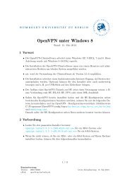
Figure 1.1. The Intel® <strong>Trace</strong> <strong>Analyzer</strong><br />
Starting the Intel® <strong>Trace</strong> <strong>Analyzer</strong><br />
Note<br />
For a proper functioning of the Intel <strong>Trace</strong> <strong>Analyzer</strong> you must ensure that<br />
files do not get modified while they are opened in the <strong>Trace</strong> <strong>Analyzer</strong>.<br />
Starting in a UNIX* Environment<br />
In a UNIX* environment, invoke the Intel <strong>Trace</strong> <strong>Analyzer</strong> via the command line<br />
by typing<br />
Document number: 318120-002 1
Intel® <strong>Trace</strong> <strong>Analyzer</strong> <strong>User's</strong> <strong>Reference</strong> <strong>Guide</strong><br />
$ traceanalyzer<br />
Assuming that the executable is found, this command launches the Intel <strong>Trace</strong><br />
<strong>Analyzer</strong>. Optionally, one or more trace files are specified as arguments as shown<br />
in the following example:<br />
$ traceanalyzer poisson_icomm.single.stf &<br />
The above example opens the trace file poisson_icomm.single.stf in the Intel<br />
<strong>Trace</strong> <strong>Analyzer</strong> (See Figure 1.1, “The Intel® <strong>Trace</strong> <strong>Analyzer</strong>”). To open trace<br />
files within the Intel <strong>Trace</strong> <strong>Analyzer</strong> without restarting it, use the File Menu<br />
entry Main Menu → File → Open. Each time a trace file is opened a new window<br />
displaying the trace file's Function Profile Chart is displayed (See Figure 1.2,<br />
“poisson_sendrecv.single.stf loaded”).<br />
Starting in a Windows* Environment<br />
In a Windows* environment, double-click on a trace file to invoke the Intel <strong>Trace</strong><br />
<strong>Analyzer</strong> or use the menu item Start → All Programs → Intel <strong>Trace</strong> <strong>Analyzer</strong>.<br />
The <strong>Trace</strong> Cache<br />
For every trace file opened by the Intel <strong>Trace</strong> <strong>Analyzer</strong>, a trace cache is created<br />
for more efficient access. It is stored in the same directory as the trace file and<br />
has the same filename but with the suffix .cache added.<br />
The Command Line Interface (CLI)<br />
The Intel <strong>Trace</strong> <strong>Analyzer</strong> provides a command line interface (CLI) in the Windows*<br />
and the UNIX* environment. One application of the CLI is to pre-calculate trace<br />
caches for new trace files from batch files without invocation of the graphical<br />
user interface. This might be useful for very big tracefiles. You might also want<br />
to automate producing profiling data for several tracefiles without further user<br />
interaction. For details refer to Chapter 8, Command Line Interface (CLI).<br />
Internationalization<br />
Intel <strong>Trace</strong> <strong>Analyzer</strong>'s target audience is pretty small compared to, say a word<br />
processor and the same installation on a parallel computer will often be used<br />
in diverse communities. The GUI is as agnostic as possible when it comes to<br />
internationalization (or i18n for short).<br />
There is only an English version of the software and the documentation. Also, the<br />
number formats in the GUI (refer to the section called “The Style Menu” and the<br />
section called “Number Formatting Settings”) and in exported text files always<br />
use a decimal point and when separating three digit groups a space character is<br />
used instead of a comma or point.<br />
The problem of non-ASCII characters in path and filenames is a little more<br />
complicated. Intel <strong>Trace</strong> <strong>Analyzer</strong> uses UTF-8 encoding internally and in its<br />
configuration file to be able to deal with file and path names that contain<br />
characters from most languages of the world.<br />
Since Windows* uses the same encoding (UTF-16) in file and path names<br />
regardless of your language and region settings you do not need to configure<br />
anything to make the Intel <strong>Trace</strong> <strong>Analyzer</strong> work in your environment. As soon<br />
as the file names appear correctly in the directory listings they will be usable in<br />
the Intel <strong>Trace</strong> <strong>Analyzer</strong>.<br />
Document number: 318120-002 2
Intel® <strong>Trace</strong> <strong>Analyzer</strong> <strong>User's</strong> <strong>Reference</strong> <strong>Guide</strong><br />
On Linux* systems you will have to set the encoding part in your locale settings<br />
correctly to be able to open your tracefiles. If you use plain ASCII in your path<br />
names then you are already done. On a recent Linux* system chances are high<br />
that everything is setup correctly out of the box.<br />
Valid locale settings look like en_US.latin-1 (for an U.S. American),<br />
de_DE.UTF-8 (for a German), fr_CA.iso88591 (for a French-speaking Canadian)<br />
and ja_JP.ujis (for a Japanese). The command locale will help to list all<br />
available locales and encodings on your system. For the <strong>Trace</strong> <strong>Analyzer</strong> only the<br />
encoding part of the locale setting is relevant. All file names and path names given<br />
on the command line and read from the file system are expected to be encoded<br />
in the encoding given by the locale settings. Beware: having for example UTF-8<br />
encoded directory names and storing trace files there with ISO-8859-1 encoded<br />
filenames can lead to inaccessible files.<br />
The Intel <strong>Trace</strong> <strong>Analyzer</strong> supports the following encodings (but use the encoding<br />
names as given by locale -m):<br />
• Latin1<br />
• Big5 -- Chinese<br />
• Big5-HKSCS -- Chinese<br />
• eucJP -- Japanese<br />
• eucKR -- Korean<br />
• GB2312 -- Chinese<br />
• GBK -- Chinese<br />
• GB18030 -- Chinese<br />
• JIS7 -- Japanese<br />
• Shift-JIS -- Japanese<br />
• TSCII -- Tamil<br />
• utf8 -- Unicode, 8-bit<br />
• utf16 -- Unicode<br />
• KOI8-R -- Russian<br />
• KOI8-U -- Ukrainian<br />
• ISO8859-1 -- Western<br />
• ISO8859-2 -- Central European<br />
• ISO8859-3 -- Central European<br />
• ISO8859-4 -- Baltic<br />
• ISO8859-5 -- Cyrillic<br />
• ISO8859-6 -- Arabic<br />
• ISO8859-7 -- Greek<br />
• ISO8859-8 -- Hebrew, visually ordered<br />
• ISO8859-8-i -- Hebrew, logically ordered<br />
• ISO8859-9 -- Turkish<br />
Document number: 318120-002 3
Intel® <strong>Trace</strong> <strong>Analyzer</strong> <strong>User's</strong> <strong>Reference</strong> <strong>Guide</strong><br />
• ISO8859-10<br />
• ISO8859-13<br />
• ISO8859-14<br />
• ISO8859-15 -- Western<br />
• IBM 850<br />
• IBM 866<br />
• CP874<br />
• CP1250 -- Central European<br />
• CP1251 -- Cyrillic<br />
• CP1252 -- Western<br />
• CP1253 -- Greek<br />
• CP1254 -- Turkish<br />
• CP1255 -- Hebrew<br />
• CP1256 -- Arabic<br />
• CP1257 -- Baltic<br />
• CP1258<br />
• TIS-620 -- Thai<br />
Summary: to make your life simple when moving trace files between different<br />
systems and sharing them among people it is recommended that you use pure<br />
ASCII characters in path and file names as much as possible. When using non-<br />
ASCII characters in path names seems unavoidable then use UTF-8 encoding on<br />
Linux* since it is space efficient, can express nearly all languages, is supported<br />
on most systems and it is identical to 7bit ASCII encoding for codes 0 to 127.<br />
Online Resources<br />
Additional information about Intel® <strong>Trace</strong> <strong>Analyzer</strong> for Linux* and<br />
related products is available at: http://support.intel.com/support/<br />
performancetools/cluster/analyzer/lin/index.htm<br />
Additional information about Intel® <strong>Trace</strong> <strong>Analyzer</strong> for Windows* and<br />
related products is available at: http://support.intel.com/support/<br />
performancetools/cluster/analyzer/win/index.htm<br />
Intel® Premier support is available at: https://premier.intel.com/<br />
For the Impatient<br />
This section provides a quick start into the Intel <strong>Trace</strong> <strong>Analyzer</strong>. It<br />
demonstrates essential features of the program using the example trace<br />
files poisson_sendrecv.single.stf and poisson_icomm.single.stf that are<br />
available in the Intel <strong>Trace</strong> <strong>Analyzer</strong>'s examples directory.<br />
The traces were generated with two implementations of the same algorithm<br />
computing the same result over the same data set: a poisson solver for a<br />
linear equation system. As the names imply, the first version uses a sendrecv to<br />
communicate, while the second version uses non-blocking communication.<br />
Document number: 318120-002 4
Intel® <strong>Trace</strong> <strong>Analyzer</strong> <strong>User's</strong> <strong>Reference</strong> <strong>Guide</strong><br />
It is illustrated that the first version leads to an overall serialization of the<br />
parallel algorithm and how the improved version solves the problem. Figure 1.2,<br />
“poisson_sendrecv.single.stf loaded” shows the Intel <strong>Trace</strong> <strong>Analyzer</strong> after loading<br />
poisson_sendrecv.single.stf. The figure shows a main window and a child<br />
window, a so called View.<br />
Figure 1.2. poisson_sendrecv.single.stf loaded<br />
Maximize the View with the respective button in its title bar and open an Event<br />
Timeline (View Menu → Charts → Event Timeline) as shown in Figure 1.3, “Opening<br />
an Event Timeline”. The result should look like in Figure 1.4, “Event Timeline<br />
opened”.<br />
Figure 1.3. Opening an Event Timeline<br />
Figure 1.4. Event Timeline opened<br />
Document number: 318120-002 5
Intel® <strong>Trace</strong> <strong>Analyzer</strong> <strong>User's</strong> <strong>Reference</strong> <strong>Guide</strong><br />
Together with the Event Timeline (see the section called “Event Timeline”), a time<br />
scale opens above the Timeline in the View. Figure 1.4, “Event Timeline opened”<br />
shows a View containing a time scale, an Event Timeline and a Function Profile.<br />
These diagrams are called Charts (see Chapter 4, Charts). In the status bar (see<br />
the section called “The Status Bar”) found at the bottom of the View the current<br />
time interval and some other information are shown.<br />
Zoom into the interesting area on the right edge of the Event Timeline by dragging<br />
the mouse over the desired time interval with the left mouse button pressed<br />
as shown in Figure 1.5, “Zooming into a Chart”. The result should look like in<br />
Figure 1.6, “Zoomed result”. Note the apparent iterative nature of the application.<br />
Figure 1.5. Zooming into a Chart<br />
Figure 1.6. Zoomed result<br />
Now zoom further into the trace to look at a single iteration and close the Function<br />
Profile (Context Menu → Close Chart). The result should look like Figure 1.7,<br />
“Zoomed to one iteration”.<br />
Document number: 318120-002 6
Intel® <strong>Trace</strong> <strong>Analyzer</strong> <strong>User's</strong> <strong>Reference</strong> <strong>Guide</strong><br />
Figure 1.7. Zoomed to one iteration<br />
To see which particular MPI functions are used in the program, right-click on<br />
MPI in the Event Timeline and choose Ungroup Group MPI. The result should<br />
look like Figure 1.8, “MPI ungrouped ”. The Function Aggregation of the View<br />
changes so that the MPI functions are no longer aggregated (see the section<br />
called “Aggregation”) into the Function Group MPI but are shown individually. This<br />
is shown in the status bar. The button titled Major Function Groups changes to<br />
MPI expanded in (Major Function Groups). Click this button to open the Function<br />
Group Editor (see the section called “The Function Group Editor”), which enables<br />
you to create new function groups and to switch between them.<br />
Figure 1.8. MPI ungrouped<br />
It is apparent that at the start of the iteration the processes communicate<br />
with their direct neighbors using MPI_Sendrecv. The way this data exchange is<br />
implemented shows a clear disadvantage: process i does not exchange data with<br />
its neighbor i+1 until the exchange between i-1 and i is complete. This makes<br />
the first MPI_Sendrecv block look like a staircase. The second block is already<br />
deferred and hence does not show the same effect. The MPI_Allreduce at the<br />
end of the iteration nearly resynchronizes all processes. The net effect is that the<br />
processes spend most of their time waiting for each other.<br />
Looking at the status bar (see Figure 1.8, “MPI ungrouped ”) shows that one<br />
iteration is roughly 1.5 milliseconds long.<br />
Figure 1.9, “Many Charts” shows a View with an Event Timeline (View Menu →<br />
Charts → Event Timeline), two Function Profiles (View Menu → Charts → Function<br />
Profile) with their Load Balance tab and a Message profile (View Menu → Charts<br />
→ Message Profile) that reveals the asymmetric pattern in the point to point<br />
messages.<br />
Document number: 318120-002 7
Intel® <strong>Trace</strong> <strong>Analyzer</strong> <strong>User's</strong> <strong>Reference</strong> <strong>Guide</strong><br />
Note that the time spent in MPI_Sendrecv grows with the process number while<br />
the time for MPI_Allreduce decreases. The Message Profile (the section called<br />
“The Message Profile”) in the bottom right corner of Figure 1.9, “Many Charts”<br />
shows that messages traveling from a higher rank to a lower rank need more and<br />
more time with increasing rank while the messages traveling from lower rank to<br />
higher rank do reveal a weak even-odd kind of pattern.<br />
Figure 1.9. Many Charts<br />
As poisson_sendrecv.single.stf is such a striking example of serialization,<br />
next to all Charts provided by the Intel <strong>Trace</strong> <strong>Analyzer</strong> reveal this interesting<br />
pattern. But in real world cases it might be necessary to formulate a hypothesis<br />
regarding how the program should behave and to check this hypothesis using<br />
the most adequate Chart.<br />
A possible way to improve the performance of the program is to use nonblocking<br />
communication to replace the usage of MPI_Sendrecv and to avoid the<br />
serialization in this way. One iteration of the resulting program looks like the one<br />
shown in Figure 1.10, “One iteration of the improved version”. Note that a single<br />
iteration now takes about 0.9 milliseconds, while it took about 1.4 milliseconds<br />
before the change.<br />
Figure 1.10. One iteration of the improved version<br />
To compare two trace files the Intel <strong>Trace</strong> <strong>Analyzer</strong> offers the so called<br />
Comparison View (see Chapter 7, Comparison of two <strong>Trace</strong> Files). Just<br />
use the menu entry View Menu → View → Compare in the View showing<br />
poisson_sendrecv.single.stf. In the now appearing dialog choose another<br />
Document number: 318120-002 8
Intel® <strong>Trace</strong> <strong>Analyzer</strong> <strong>User's</strong> <strong>Reference</strong> <strong>Guide</strong><br />
View that shows poisson_icomm.single.stf. A new Comparison View is opened<br />
that shows an Event Timeline for each file and a Comparison Function Profile<br />
Chart (see the section called “The Comparison Function Profile”) that shows a<br />
profile computed from both tracefiles. The time intervals, aggregation settings<br />
and filters are taken from the original Views.<br />
After adjusting some configurable behavior (see Chapter 7, Comparison of two<br />
<strong>Trace</strong> Files) and zooming to the first iteration in each trace file a Comparison View<br />
for these two files can look like in Figure 1.11, “Comparing the first iterations<br />
taken from two program runs”. Now it is immediately obvious that one iteration in<br />
the improved program needs considerable less time than in the original program.<br />
Figure 1.11. Comparing the first iterations taken from two<br />
program runs<br />
Please note that you can create a Comparison View that compares one time<br />
interval and one process group against another time interval and another process<br />
group of the same trace file. Other useful applications of the Comparison View<br />
include scalability analysis where you compare two runs of the same unmodified<br />
program with different processor counts and try to find out which functions scale<br />
well and which suffer from Amdahls Law. Other scenarios could be the comparison<br />
of two different MPI libraries, interconnects or machines.<br />
Of course this introduction only scratches the surface. If there is not enough<br />
time to browse through the whole documentation, it is recommended to at least<br />
read through Chapter 10, Concepts to learn about features like filtering, tagging,<br />
process aggregation and function aggregation. These features have the potential<br />
to make analyzing parallel applications more efficient.<br />
Document number: 318120-002 9
Intel® <strong>Trace</strong> <strong>Analyzer</strong> <strong>User's</strong> <strong>Reference</strong> <strong>Guide</strong><br />
Chapter 2. The Main Menu<br />
The main menu of the Intel® <strong>Trace</strong> <strong>Analyzer</strong> contains options using which the<br />
general settings of the <strong>Analyzer</strong> can be changed. Use these entries to edit the<br />
configuration settings and the display style.<br />
There are four sub-menus in the main menu. These are:<br />
1. File Menu<br />
2. Style Menu<br />
3. The Windows* Menu<br />
4. Help Menu<br />
The File Menu<br />
The File menu has four entries. The Open menu entry opens a dialog. Specify one<br />
or several trace files to open in this dialog.<br />
Figure 2.1. The File Menu<br />
To select a new configuration, use the Load Configuration entry. This opens a<br />
dialog where the required configuration is selected.<br />
The option Edit Configuration opens the Configuration dialog which is explained<br />
in the section called “The Edit Configuration Dialog”.<br />
The Quit entry exits the Intel <strong>Trace</strong> <strong>Analyzer</strong>. Below the Quit entry, there is a list<br />
of the ten trace files opened most recently.<br />
The Style Menu<br />
The Style menu provides the option of choosing the design in which the view is<br />
displayed. The options in the Style menu depend on the environment in use. The<br />
first entry always shows the default style for the respective platform (or for the<br />
respective window manager when using X Windows). For example, in a Windows*<br />
environment, the user has the option of choosing between the QWindowsXPStyle<br />
option, the Windows option and the WindowsXP option. In a KDE environment,the<br />
user has the default as QMotifStyle and CDE, Motif, MotifPlus, Platinum, SGI and<br />
Windows as other options.<br />
Additional styles may be available when provided by a desktop environment like<br />
KDE. If you experience problems with those styles then switch back to the default<br />
Document number: 318120-002 10
Intel® <strong>Trace</strong> <strong>Analyzer</strong> <strong>User's</strong> <strong>Reference</strong> <strong>Guide</strong><br />
style. There will be no support in case of problems that cannot be reproduced<br />
using the default style.<br />
Figure 2.2. The Style Menu<br />
Figure 2.3. The Style Menu on Windows*<br />
• Set Fonts<br />
Use the Set Fonts option to change the fonts in the Intel <strong>Trace</strong> <strong>Analyzer</strong>. A<br />
dialog opens where the fonts can be changed for the individual Charts. For more<br />
information on the Font dialog box refer to the section called “Font Settings”.<br />
• Number Formatting<br />
This option lets you specify the format of the various numerical values displayed<br />
in the Intel <strong>Trace</strong> <strong>Analyzer</strong>. For more information on Number Formatting, refer<br />
to the section called “Number Formatting Settings”.<br />
The Windows Menu<br />
Use the menu options in the Windows menu to arrange the open sub-windows as<br />
required. There are three possibilities which are explained below. The Windows<br />
sub-menu also shows the name and path of the trace file that is presently opened.<br />
• Cascade<br />
Select the Cascade option to arrange the open sub-windows one behind the<br />
other.<br />
• Tile<br />
The Tile option arranges the sub-windows next to each other. Note that this<br />
option is useful only when charts are opened in two or more sub-windows.<br />
• Iconify<br />
Iconify minimizes the open sub-windows and shows the icon of these in the<br />
bottom of the View.<br />
Document number: 318120-002 11
Intel® <strong>Trace</strong> <strong>Analyzer</strong> <strong>User's</strong> <strong>Reference</strong> <strong>Guide</strong><br />
Figure 2.4. The Windows Menu<br />
The Help Menu<br />
The Help allows you to access the HTML formatted online help via an integrated<br />
HTML browser. The first entry points to the table of contents while the next two<br />
point to a section about online resources.<br />
The help is also installed in PDF format to ease printing.<br />
The last entry gives you details regarding the Intel <strong>Trace</strong> <strong>Analyzer</strong> in use.<br />
Throughout the application context sensitive help for the current Chart, dialog<br />
box or context menu is available by pressing F1.<br />
Document number: 318120-002 12
Intel® <strong>Trace</strong> <strong>Analyzer</strong> <strong>User's</strong> <strong>Reference</strong> <strong>Guide</strong><br />
Chapter 3. Views<br />
For a flexible analysis of a trace file it is helpful to look at multiple partitions of<br />
the data from various perspectives. The concept of Views is introduced here. A<br />
View holds a collection of Charts in a single window. These Charts, inherent in<br />
the same View, use the same perspective on the data. This perspective is made<br />
up of the following attributes: the time interval, process aggregation, function<br />
aggregation and filters. For an in-depth explanation of aggregation and filters,<br />
refer to Chapter 10, Concepts.<br />
Whenever an attribute in the current perspective is changed for one of the Charts,<br />
all other Charts follow. Opening several Views offers a very flexible and variable<br />
mechanism for exploring, analyzing and comparing trace data. The View's status<br />
bar shows the current perspective on the data and allows to quickly change the<br />
perspective. More about the status bar is described in the section called “The<br />
Status Bar”.<br />
The View's Main Menu<br />
All operations that can be performed on a View are found on the View's menu<br />
bar. This menu bar consists of five menu options:<br />
• View Menu<br />
• Charts Menu<br />
• Navigate Menu<br />
• Advanced Menu<br />
• Layout Menu<br />
• Comparison Menu<br />
The View Menu<br />
The View menu consists of options that are carried out on the entire View. These<br />
options are described below:<br />
Figure 3.1. The View Menu<br />
• Open New (Ctrl+Alt+O)<br />
This opens the New View dialog box, which opens a new View with the selected<br />
Charts. The New View dialog box is explained in the section called “The New<br />
View Dialog”.<br />
• <strong>Trace</strong>file Info (Ctrl+Alt+I)<br />
Document number: 318120-002 13
Intel® <strong>Trace</strong> <strong>Analyzer</strong> <strong>User's</strong> <strong>Reference</strong> <strong>Guide</strong><br />
This opens the <strong>Trace</strong>file Info dialog box, which contains the full information<br />
about the current trace.<br />
• Clone (Ctrl+Alt+D)<br />
This command replicates the existing View. It creates a one-to-one clone of<br />
the current View.<br />
• Save (Ctrl+Alt+S)<br />
This command saves the entire View as a picture.<br />
• Print (Ctrl+Alt+P)<br />
This entry prints a copy of the View.<br />
• Redraw (Ctrl+Alt+R)<br />
This command repaints the entire View.<br />
• Close (Ctrl+Alt+W)<br />
This command closes the current View. If the last View for a trace file is closed,<br />
the trace file is closed as well.<br />
• Compare<br />
This opens a dialog to select a file for comparison with the present one. This<br />
can be the current file of another trace file that is already open. After choosing<br />
the file, a new Comparison View will be opened that displays data from the two<br />
files. See Chapter 7, Comparison of two <strong>Trace</strong> Files.<br />
The Charts Menu<br />
The Charts menu contains entries to open the various Charts of the Intel® <strong>Trace</strong><br />
<strong>Analyzer</strong>. There are seven entries in this menu:<br />
Figure 3.2. The Charts Menu<br />
• TimeScale<br />
This TimeScale entry displays the Timescale. The Timescale also appears<br />
automatically on first opening of any Timeline Chart.<br />
• Event Timeline (Ctrl+Alt+E)<br />
The Event Timeline is a Chart that visualizes what the individual processes are<br />
doing. The Event Timeline is explained in detail in the section called “Event<br />
Timeline”.<br />
Document number: 318120-002 14
Intel® <strong>Trace</strong> <strong>Analyzer</strong> <strong>User's</strong> <strong>Reference</strong> <strong>Guide</strong><br />
• Qualitative Timeline (Ctrl+Alt+L)<br />
The Qualitative Timeline shows event attributes as they occur over time. This<br />
timeline is explained in the section called “Qualitative Timeline”.<br />
• Quantitative Timeline (Ctrl+Alt+N)<br />
This entry opens the Quantitative Timeline. It gives an overview of the parallel<br />
behavior of the application and is explained in the section called “Quantitative<br />
Timeline”.<br />
• Counter Timeline (Ctrl+Alt+U)<br />
The Counter Timeline shows the values of all counters that are present in the<br />
trace file. For more information on the Counter Timeline, see the section called<br />
“Counter Timeline”.<br />
• Function Profile (Ctrl+Alt+F)<br />
This entry opens the Function Profile. On opening a trace file in the Intel <strong>Trace</strong><br />
<strong>Analyzer</strong>, the Function Profile is shown by default. For more information on the<br />
Function Profile, see the section called “The Function Profile Chart”.<br />
• Message Profile (Ctrl+Alt+M)<br />
The Message Profile provides statistical information on MPI point to point<br />
messages. Messages are categorized by grouping them in two dimensions. A<br />
detailed description of the Message Profile is available in the section called “The<br />
Message Profile”.<br />
• Collective Operations Profile (Ctrl+Alt+C)<br />
The Collective Operations Profile provides statistical information on MPI's<br />
collective operations. Operations are categorized by grouping them in two<br />
dimensions. For more information on the Collective Operations Profile, refer to<br />
the section called “The Collective Operations Profile”.<br />
The Navigate Menu<br />
All functions provided by the Navigation Menu are also available through<br />
convenient keyboard shortcuts. Please note that these keyboard shortcuts work<br />
only when a timeline has the keyboard focus. To give the keyboard focus to a<br />
timeline just left-click into it. The keyboard focus is indicated by a black rectangle<br />
around the timeline.<br />
The entries in the Navigate menu are:<br />
Document number: 318120-002 15
Intel® <strong>Trace</strong> <strong>Analyzer</strong> <strong>User's</strong> <strong>Reference</strong> <strong>Guide</strong><br />
Figure 3.3. The Navigate Menu<br />
• Back (B):<br />
Pops the current interval from the zoom stack (the section called “The Zoom<br />
Stack”).<br />
• Zoom In (I):<br />
Magnifies by a factor of two around the current center and pushes this new<br />
interval onto the zoom stack (the section called “The Zoom Stack”).<br />
• Zoom Out (O):<br />
Scales by a factor of 1/2 around the current center and pushes this new interval<br />
onto the zoom stack (the section called “The Zoom Stack”).<br />
• Reset Zoom (R):<br />
Clears the zoom stack and then pushes a time interval onto the zoom stack (the<br />
section called “The Zoom Stack”) that corresponds to the complete trace file.<br />
• Zoom Up (U):<br />
Maintains the current center and goes back to the previous zoom step.<br />
• Left 1/1 (Ctrl-Left):<br />
Moves one whole screen to the left and pushes the new interval onto the zoom<br />
stack (the section called “The Zoom Stack”).<br />
• Right 1/1 (Ctrl-Right):<br />
Moves one whole screen to the right and pushes the new interval onto the zoom<br />
stack (the section called “The Zoom Stack”).<br />
• Left 1/2 (Left):<br />
Moves half a screen to the left and pushes the new interval onto the zoom stack<br />
(the section called “The Zoom Stack”).<br />
• Right 1/2 (Right):<br />
Moves half a screen to the right and pushes the new interval onto the zoom<br />
stack (the section called “The Zoom Stack”).<br />
• Left 1/4 (Shift-Left):<br />
Document number: 318120-002 16
Intel® <strong>Trace</strong> <strong>Analyzer</strong> <strong>User's</strong> <strong>Reference</strong> <strong>Guide</strong><br />
Moves a quarter of a screen to the left and pushes the new interval onto the<br />
zoom stack (the section called “The Zoom Stack”).<br />
• Right 1/4 (Shift-Right):<br />
Moves a quarter of a screen to the right and pushes the new interval onto the<br />
zoom stack (the section called “The Zoom Stack”).<br />
• To Start (Home):<br />
Moves to the start of the trace file and pushes the new interval onto the zoom<br />
stack. (the section called “The Zoom Stack”)<br />
• To End (End):<br />
Moves to the end of the trace file and pushes the new interval onto the zoom<br />
stack (the section called “The Zoom Stack”).<br />
• Goto (G):<br />
Opens the Time Interval Selection dialog box (the section called “Time Interval<br />
Selection”).<br />
The Advanced Menu<br />
Figure 3.4. The Advanced Menu<br />
• Tagging<br />
Tagging highlights events that satisfy specific user-defined conditions. Click on<br />
this entry to open the dialog box where the tagging conditions are specified.<br />
For more information on the Tagging dialog box. refer to the section called “The<br />
Tagging Dialog”.<br />
• Filtering<br />
Filtering shows only those events that satisfy a condition as defined by the<br />
user. All other events are suppressed as if they had never been written to the<br />
trace file. The filtering dialog box is explained in the section called “The Filtering<br />
Dialog”.<br />
• Reset Tagging/Filtering<br />
This menu entry is active only when the chart has been either filtered or tagged.<br />
It undoes the tagging/filtering. All events are shown and none are filtered or<br />
tagged.<br />
• Process Aggregation<br />
Document number: 318120-002 17
Intel® <strong>Trace</strong> <strong>Analyzer</strong> <strong>User's</strong> <strong>Reference</strong> <strong>Guide</strong><br />
Process Aggregation focusses on the processes that are of importance to<br />
the user and aggregates the results to Process Groups. It accesses the<br />
Process Group Editor (the section called “The Process Group Editor”) where the<br />
appropriate process groups can be constructed and/or chosen.<br />
• Function Aggregation<br />
Function Aggregation focuses on a subset of functions and aggregates these<br />
into Function Groups, without being distracted by other functions that are<br />
currently not significant to the user. Use the Function Group Editor (the section<br />
called “The Function Group Editor”) to do this.<br />
• Default Aggregation<br />
Default aggregation sets the aggregation values back to the default settings<br />
which are All Processes for process aggregation and Major Function Groups for<br />
function aggregation.<br />
• Show Process Group “Other”<br />
If the process aggregation does not cover all processes present in the trace file<br />
then all data for uncovered processes are subsumed in the artificially created<br />
process group Other.<br />
Use this switch to show or hide the process group Other. The default is to hide<br />
this group.<br />
The Quantitative Timeline and the Function Profile allow selecting a subset of<br />
the current processes to be shown and can hence override this switch.<br />
• Show Function Group “Other”<br />
If the current function aggregation does not cover all functions in the trace<br />
file then all uncovered function events are subsumed in the artificially created<br />
function group Other.<br />
Use this switch to show or hide this group. By default, the switch is enabled<br />
to show this group.<br />
The Event Timeline always shows the Function Group Other wherever applicable<br />
instead of showing “holes”. The Quantitative Timeline and the Function Profile<br />
enable selecting a subset of the current functions to be shown and can therefore<br />
override this switch.<br />
The Layout Menu<br />
Generally, every View is split into two sections: one for timelines and the other<br />
for Profiles. The Layout menu adjusts the position of the Charts or the respective<br />
sections on screen. For example, it provides the option of viewing the timelines<br />
and profiles next to each other or like the default, one below the other. The<br />
different entries of the layout menu, which are enabled when two or more charts<br />
are open, are explained below.<br />
Document number: 318120-002 18
Intel® <strong>Trace</strong> <strong>Analyzer</strong> <strong>User's</strong> <strong>Reference</strong> <strong>Guide</strong><br />
Figure 3.5. The Layout Menu<br />
• Timelines to Top<br />
Use this entry to move the timelines to the upper portion of the View and the<br />
profiles to the bottom.<br />
• Timelines to Bottom<br />
Use this entry to move the timelines to the lower portion of the View and the<br />
profiles to the top.<br />
• Timelines to Left<br />
Use this entry to place the timelines to the left of the View. For example, to<br />
display the Charts next to each other, select the option View Menu → Layout<br />
→ Timelines to Left. This moves the timeline(s) being shown in the View to<br />
the left of the screen, and thereby also shifts the profiles being shown to the<br />
other side. In case multiple timelines are open, these are collectively shown<br />
one below the other on the chosen side.<br />
• Timelines to Right<br />
Use this entry to place all the timelines to the right of the View. It works the<br />
same way as Timelines to Left.<br />
Figure 3.6. Placing timelines to the right<br />
• Swap Layout of Timelines<br />
Swaps the position of the timelines relative to each other. It is useful only when<br />
two or more timelines are open at the same time. If the timelines are stacked<br />
and aligned on top of each other, use this option to present them next to each<br />
other (or vice versa). The menu entry switches between the two choices.<br />
• Swap Layout of Profiles<br />
Document number: 318120-002 19
Intel® <strong>Trace</strong> <strong>Analyzer</strong> <strong>User's</strong> <strong>Reference</strong> <strong>Guide</strong><br />
Swaps the position of the profiles relative to each other, similar to that of the<br />
timelines as explained above.<br />
• Default Layout<br />
This option brings the layout of the View back to the default settings. By default,<br />
timelines are stacked in the upper portion of the View and Profiles in the lower<br />
portion, side by side.<br />
The Comparison Menu<br />
The Comparison menu is displayed in the Views menu only when the Comparison<br />
mode is activated (View Menu → Compare). This menu has four entries which are<br />
explained in Chapter 7, Comparison of two <strong>Trace</strong> Files.<br />
The Status Bar<br />
When moving the mouse cursor over an event in a timeline or an entry in a profile,<br />
expanded information on the respective entry is seen in the status bar at the<br />
bottom of the View for a few seconds. After this, or when the mouse moves into<br />
the status bar, it provides buttons that show the current settings and that enable<br />
changing the current settings. These shortcut buttons are described below:<br />
• Time Interval<br />
The leftmost button in the status bar opens a dialog box that sets the time<br />
interval. More about the time interval dialog box is available in the section called<br />
“Time Interval Selection”. The title on this button is of the form “$Start, $End:<br />
$Duration”. The status bar in Figure 3.6, “Placing timelines to the right” shows<br />
that the start position of the time interval is at 0.0 seconds, the end position<br />
at 2.072 seconds and that the duration is 2.072 seconds. The button appears<br />
flat when the full time range of the file is shown.<br />
• Sec./Tick<br />
This button shows the current unit of time and switches the unit from seconds<br />
to ticks and vice versa. The button appears flat if the unit in use is seconds and<br />
appears raised when using ticks.<br />
• Process Aggregation<br />
This button shows the current process aggregation. By default, this is<br />
All_Processes. Click this button to open the Process Group Editor dialog box,<br />
which is explained in the section called “The Process Group Editor”. The button<br />
appears flat for the default process aggregation.<br />
• Function Aggregation<br />
This button shows the current function aggregation. Per default, this is Major<br />
Function Groups. Clicking this button opens the Function Group Editor dialog<br />
box, which is explained in the section called “The Function Group Editor”. The<br />
button appears flat for the default function aggregation.<br />
• Tagging and Filtering<br />
The buttons labeled Tag and Filter open the Tagging dialog box (see the section<br />
called “The Tagging Dialog”) and the Filtering dialog box (see the section called<br />
Document number: 318120-002 20
Intel® <strong>Trace</strong> <strong>Analyzer</strong> <strong>User's</strong> <strong>Reference</strong> <strong>Guide</strong><br />
“The Filtering Dialog”) respectively. These buttons appear flat if no tagging/<br />
filtering is selected.<br />
Navigation In Time<br />
In addition to the menu entries and keystrokes mentioned in the section called<br />
“The Navigate Menu”, there are two more ways to move in time in the Intel <strong>Trace</strong><br />
<strong>Analyzer</strong>. One is by using the scroll bar found below the timelines and another is<br />
by using the mouse to zoom into a time interval. Similar to the keystrokes, these<br />
operations manipulate the zoom stack. Refer to the section called “The Zoom<br />
Stack” for a detailed explanation.<br />
To move the View by a quarter of a screen to a selected direction, click on the<br />
arrow buttons of the scroll bar. To move the View by one entire screen, click into<br />
the bar. Both actions push the new interval onto the zoom stack.<br />
To use the mouse for zooming, left-click into the timeline (even clicking into the<br />
Timescale works) and select the region of the new time interval, keeping the left<br />
mouse button pressed. On releasing the left mouse button this new interval is<br />
pushed onto the zoom stack.<br />
Figure 3.7. Zooming with the mouse<br />
The Zoom Stack<br />
The zoom stack supports navigation in time by storing previously displayed time<br />
intervals. These time intervals are restored when required. Navigation using the<br />
keyboard or mouse is quite intuitive without detailed knowledge of the zoom<br />
stack. Nevertheless, an explanation is given below for the sake of complete<br />
reference.<br />
Consider a trace file spanning the time from 0 to 100 seconds. When the first<br />
View is opened the zoom stack looks like this:<br />
Figure 3.8. The zoom stack<br />
0:(0;100)(50;100)<br />
Each stack entry has the syntax (Start; Stop)(Center; Width). Zooming in using<br />
I (Zoom In), magnifies the Chart by a factor of 2 around the current center.In the<br />
above example, the center is at 50 seconds. Therefore, zooming in twice using I<br />
will result in a stack as shown in Figure 3.9, “State of the zoom stack - Zoomed<br />
in twice”.<br />
Document number: 318120-002 21
Intel® <strong>Trace</strong> <strong>Analyzer</strong> <strong>User's</strong> <strong>Reference</strong> <strong>Guide</strong><br />
Figure 3.9. State of the zoom stack - Zoomed in twice<br />
3:(55;65)(60;10)<br />
2:(50;70)(60;20)<br />
1:(40;80)(60;40)<br />
0:(0;100)(50;100)<br />
Figure 3.9, “State of the zoom stack - Zoomed in twice” shows that a stack level is<br />
created for each action performed. On pressing Ctrl+Right twice, the time frame<br />
of the Chart is moved to the right by two window sizes. Using the state shown<br />
in Figure 3.10, “State of the zoom stack - Moved two window sizes to the right”,<br />
the differences between Back (B), Zoom Out (O) and Zoom Up (U) are explained<br />
below.<br />
Figure 3.10. State of the zoom stack - Moved two window<br />
sizes to the right<br />
5:(75;85)(80;10)<br />
4:(65;75)(70;10)<br />
3:(55;65)(60;10)<br />
2:(50;70)(60;20)<br />
1:(40;80)(60;40)<br />
0:(0;100)(50;100)<br />
Back (B): Pressing B in the state shown in Figure 3.10, “State of the zoom stack<br />
- Moved two window sizes to the right” pops out one level of the stack and the<br />
previous time frame is displayed as shown in Figure 3.11, “State of the zoom<br />
stack - after Back (B)”.<br />
Figure 3.11. State of the zoom stack - after Back (B)<br />
4:(65;75)(70;10)<br />
3:(55;65)(60;10)<br />
2:(50;70)(60;20)<br />
1:(40;80)(60;40)<br />
0:(0;100)(50;100)<br />
Zoom Out: Using O in Figure 3.10, “State of the zoom stack - Moved two window<br />
sizes to the right” lowers the magnification (doubles the width) and pushes a<br />
new item on the stack. Zooming out using O in the state shown in Figure 3.10,<br />
“State of the zoom stack - Moved two window sizes to the right” results in the<br />
stack as shown below.<br />
Figure 3.12. State of the zoom stack - after Zoom Out (O)<br />
6:(70;90)(80;20)<br />
5:(75;85)(80;10)<br />
4:(65;75)(70;10)<br />
3:(55;65)(60;10)<br />
2:(50;70)(60;20)<br />
1:(40;80)(60;40)<br />
0:(0;100)(50;100)<br />
Zoom Up (U): The resultant zoom after using U is a little more complicated.<br />
Pressing U keeps the current center and uses the magnification from before the<br />
Document number: 318120-002 22
Intel® <strong>Trace</strong> <strong>Analyzer</strong> <strong>User's</strong> <strong>Reference</strong> <strong>Guide</strong><br />
latest "zoom in" (which is the change from level 2 to 3 in Figure 3.10, “State of<br />
the zoom stack - Moved two window sizes to the right”) and to clear the stack up<br />
to and including the last "zoom in" found. In our example the current center is<br />
80 and the width from stack level 2, which is 20, is used.<br />
Figure 3.13. State of the zoom stack - after Zoom Up (U)<br />
2:(70;90)(80;20)<br />
1:(40;80)(60;40)<br />
0:(0;100)(50;100)<br />
Reset (R) : Reset clears the stack and pushes one entry covering the full time<br />
range of the trace file. Therefore, on pressing R, the stack shown in Figure 3.8,<br />
“The zoom stack” is reestablished.<br />
Document number: 318120-002 23
Intel® <strong>Trace</strong> <strong>Analyzer</strong> <strong>User's</strong> <strong>Reference</strong> <strong>Guide</strong><br />
Chapter 4. Charts<br />
Charts in the Intel® <strong>Trace</strong> <strong>Analyzer</strong> are graphical or alphanumerical diagrams<br />
that are parameterized with a time interval, a process grouping and a function<br />
grouping (see the section called “Aggregation”) and an optional filter. Together<br />
they define the structure in which data is presented and the amount of data to<br />
be displayed.<br />
The Charts supported by the Intel <strong>Trace</strong> <strong>Analyzer</strong> is divided into:<br />
1. Timelines: the Event Timeline, the Qualitative Timeline, the Quantitative<br />
Timeline and the Counter Timeline.<br />
2. Profiles: the Function Profile, the Message Profile and the Collective Operations<br />
Profile.<br />
Charts are grouped into Views. These Views provide ways to choose the time<br />
interval, the process grouping and optional filters that all Charts in the View use.<br />
For more details on Views, refer to Chapter 3, Views.<br />
While the former show trace data in graphical form over a horizontal axis<br />
representing runtime, the latter show statistical data. All these Charts are found<br />
under Views Menu → Charts. Opening a file in the Intel <strong>Trace</strong> <strong>Analyzer</strong>, displays<br />
a View containing the Function Profile Chart (showing the Flat Profile tab) for the<br />
opened file.<br />
The following sections describe each Chart in detail. For each Chart there is a<br />
subsection about Mouse Hovering, the context menu, the settings dialog box, the<br />
effects of filtering and tagging and the effects of aggregation, if it is applicable.<br />
Event Timeline<br />
The Event Timeline provides a graphical display of the individual process'<br />
activities.<br />
Figure 4.1. The Event Timeline<br />
The horizontal axis represents an interval of the runtime of the inspected<br />
program. Vertical bars show the function in which the process is. The bars consist<br />
of rectangles labeled with the current function's name and in its color. Black lines<br />
Document number: 318120-002 24
Intel® <strong>Trace</strong> <strong>Analyzer</strong> <strong>User's</strong> <strong>Reference</strong> <strong>Guide</strong><br />
indicate messages sent between processes; they connect the sender and receiver<br />
processes.Blue lines, forming a grid, represent collective operations, such as<br />
broadcast or reduce operations. The status bar at the bottom of this panel shows<br />
information on events under the mouse cursor. By default, the entire runtime of<br />
the trace is visible. To get a better impression on the visualization primitives, use<br />
zooming. Zooming and navigation are explained in detail in the section called<br />
“The Navigate Menu”.<br />
Mouse Hover<br />
When the mouse pointer hovers over the Event Timeline, its exact position in<br />
terms of time is shown in the status bar. The status bar also shows which function,<br />
collective operations or messages are under the mouse cursor at the moment.<br />
The status bar of the Event Timeline Chart in Figure 4.1, “The Event Timeline”,<br />
shows that the mouse is currently at 2.01214 seconds over a message from P13<br />
to P14.<br />
Event Timeline Settings<br />
Use the Event Timeline Settings to change the display settings, the layout settings<br />
and the colors of the Event Timeline Chart. The display options, which are enabled<br />
using check boxes, include<br />
• Process Labels: Displays the name of the process or process group to the left.<br />
• Function Labels: Displays the name of the function or function group inside the<br />
colored bars<br />
• Timescale at top: Displays a timescale above the Chart<br />
• Timescale at bottom: Displays a timescale below the Chart<br />
• Messages over Collective Operations: This specifies what is drawn first. If<br />
enabled, messages are drawn over the collective operations such that the<br />
messages are seen and the collective operations are concealed. If disabled, the<br />
collective operations are drawn over the messages.<br />
• Use thick Lines for Messages: Displays messages using thick lines<br />
• Use thick Lines for Collective Operations: Displays collective operations using<br />
thick lines<br />
Document number: 318120-002 25
Intel® <strong>Trace</strong> <strong>Analyzer</strong> <strong>User's</strong> <strong>Reference</strong> <strong>Guide</strong><br />
Figure 4.2. Settings dialog box for the Event Timeline<br />
The Layout option consists of two sliders and two check boxes. The slider Minimal<br />
Spacing Between Bars adjusts the space between the function bars. The slider<br />
Minimal Bar Height adjusts the height of the function bar itself. For both, the unit<br />
is pixels.<br />
The Adjust Minimal Bar Height to Labels check box alters the size of the bars.<br />
Check this box to make the bars tall enough to display a function label. This<br />
option is checked by default.<br />
The check box Use Available Vertical Space influences the overall vertical layout<br />
of the bars and is also checked by default. For a better understanding, refer to<br />
Figure 4.3, “Event Timeline: Use Available Vertical Space unchecked” where the<br />
Event Timeline is shown without checking the given option and Figure 4.4, “Event<br />
Timeline: Use Available Vertical Space checked” where the Use Available Vertical<br />
Space is checked.<br />
Figure 4.3. Event Timeline: Use Available Vertical Space<br />
unchecked<br />
Document number: 318120-002 26
Intel® <strong>Trace</strong> <strong>Analyzer</strong> <strong>User's</strong> <strong>Reference</strong> <strong>Guide</strong><br />
Figure 4.4. Event Timeline: Use Available Vertical Space<br />
checked<br />
To change the colors of the functions, messages or collective operations, use the<br />
three Colors buttons at the bottom of the Settings dialog box. Function Colors<br />
call up the Function Group Color Editor (the section called “The Function Group<br />
Color Editor”). To change the color in which the messages are displayed, click on<br />
the Message Color button. This opens a dialog box where the required color is<br />
chosen. Change the color of the Collective Operations in the same way if need be.<br />
Colors chosen for messages and collectives are local to the Event Timeline Chart.<br />
Colors chosen for functions or function groups are shared by all Charts and Views<br />
belonging to the same trace file.<br />
The Context Menu<br />
Apart from the general options common to all Charts (see the section called<br />
“Common Chart Features”), the context menu of the Event Timeline provides<br />
details pertaining to the function, the message or the Collective Operation. For<br />
example, to access details about a particular message in the Event Timeline,<br />
right-click on the message and select the option Details on Message. This opens<br />
a new dialog box displaying information on sender, receiver and other message<br />
attributes. This is further explained in the section called “The Details Dialog”.<br />
When invoked for a collective operation the context menu will offer the entry<br />
Zoom to Collective that will set the View's time interval to the time covered by<br />
the respective collective operation.<br />
Figure 4.5. Event Timeline: context menu example<br />
Furthermore, the context menu has an entry to ungroup/regroup the function,<br />
which works the same way in every Chart. To display functions, messages and/<br />
or collective operations, select Show from the context menu. Select/deselect one<br />
or more of the above from the sub-menu that opens on clicking Show.<br />
Document number: 318120-002 27
Intel® <strong>Trace</strong> <strong>Analyzer</strong> <strong>User's</strong> <strong>Reference</strong> <strong>Guide</strong><br />
The context menu entries that are common to all Charts are explained in the<br />
section called “Common Chart Features”.<br />
Filtering and Tagging<br />
Tagged functions in the Event Timeline are shown with a frame around them and<br />
with the function label rendered in a bold font. Tagged messages and collectives<br />
are shown with thicker lines.<br />
Figure 4.6. Tagging functions in a process in the Event<br />
Timeline<br />
Figure 4.6, “Tagging functions in a process in the Event Timeline” shows an Event<br />
Timeline where the MPI function in process number 8 (P8) is tagged. On filtering<br />
the Event Timeline with the same clause (MPI in P8), only the MPI functions of<br />
P8 pass the filter and are displayed, while all other functions and processes are<br />
filtered out as shown in Figure 4.7, “Filtering functions in a process in the Event<br />
Timeline”. More on tagging and filtering is available in the section called “Tagging<br />
and Filtering”.<br />
Figure 4.7. Filtering functions in a process in the Event<br />
Timeline<br />
Qualitative Timeline<br />
The Qualitative Timeline (Views Menu → Charts → Qualitative Timeline) shows<br />
event attributes like the data volume of messages as they occur over time. The<br />
Document number: 318120-002 28
Intel® <strong>Trace</strong> <strong>Analyzer</strong> <strong>User's</strong> <strong>Reference</strong> <strong>Guide</strong><br />
value of this attribute is plotted along the y-axis while time is plotted along the<br />
x-axis. Select the required event type and attributes from the context menu. It<br />
helps detect patterns and irregular behavior such as extreme deviations or longterm<br />
changes in attribute values.<br />
For the Poisson example, Figure 4.8, “Qualitative Timeline” shows that the<br />
Qualitative Timeline gives a good impression of the pattern of function events<br />
Context Menu → Events to show. Zooming to a bunch of iterations again shows<br />
the staircase pattern observed above (see the section called “For the Impatient”).<br />
Showing the transfer rates for messages results in a very instructive pattern for<br />
the given trace file.<br />
A vertical line in the Qualitative Timeline either represents a single event (denoted<br />
as Single in the legend) or several events grouped together (denoted as Multi<br />
in the legend). Refer to the section called “Level of Detail” to find details on the<br />
merging of events.<br />
Figure 4.8. Qualitative Timeline<br />
Mouse Hover<br />
When the mouse hovers over the Qualitative Timeline Chart, the value of the x-<br />
axis (representing time) for the given position is shown in the status bar. The<br />
status bar also shows details regarding the given position of the mouse. For<br />
example, when the Qualitative Timeline displays the Message attribute, the status<br />
bar shows how many messages are represented at that point. In case there is<br />
only one message, the sender and the receiver of the message are displayed as<br />
well. In the case where function events are displayed, mouse hovering indicates<br />
which Function/Group is present at the given position.<br />
Document number: 318120-002 29
Intel® <strong>Trace</strong> <strong>Analyzer</strong> <strong>User's</strong> <strong>Reference</strong> <strong>Guide</strong><br />
Figure 4.9. Status Bar when the mouse hovers over the<br />
Qualitative Timeline<br />
Qualitative Timeline Settings<br />
The settings dialog box of the Qualitative Timeline consists of a Display group<br />
with check boxes and a Vertical scaling combo box. Use the combo box to adjust<br />
the vertical scaling of the timeline.<br />
Figure 4.10. The Qualitative Timeline settings dialog box<br />
Document number: 318120-002 30
Intel® <strong>Trace</strong> <strong>Analyzer</strong> <strong>User's</strong> <strong>Reference</strong> <strong>Guide</strong><br />
The Display Group specifies which scales to show and whether an own legend<br />
needs to be displayed for the timeline. By default, the vertical scale and the<br />
legend are shown.<br />
Use the Vertical Scaling group to switch between the default Automatic Scaling<br />
and the Manual Scaling of the y-axis. To explicitly specify the maximum scale<br />
value, use Manual scaling. To visually compare two or more Charts in the same<br />
or distinct Views, specify the same maximum value for the charts.<br />
Context Menu<br />
The entry Context Menu → Events to show allows to choose the event type from<br />
Function Events, Messages and Collective Ops via a sub-menu.<br />
The entry Context Menu → Attribute to show → xxx allows to choose the particular<br />
attribute value of the event from Duration, Transfer Rate or Data Volume via a<br />
sub-menu. Note that not all attributes are available for all event types.<br />
Filtering and Tagging<br />
Tagged items in the Qualitative Timeline are highlighted by coloring them red.<br />
For example, to tag all messages sent by P9, open the Tagging dialog box (the<br />
section called “The Tagging Dialog”) and go to the Messages tab.<br />
Figure 4.11. Tagging in the Qualitative Timeline<br />
Here, in the group Messages to be Tagged select the radio button titled Custom.<br />
Specify whatever needs to be tagged in the given field. Figure 4.11, “Tagging in<br />
the Qualitative Timeline” shows that P9 is tagged, resulting in the timeline shown<br />
in Figure 4.12, “Qualitative Timeline with tagged messages”.<br />
Document number: 318120-002 31
Intel® <strong>Trace</strong> <strong>Analyzer</strong> <strong>User's</strong> <strong>Reference</strong> <strong>Guide</strong><br />
Figure 4.12. Qualitative Timeline with tagged messages<br />
Similarly, to filter out all messages except those sent by P9, use the Filtering<br />
dialog box (the section called “The Filtering Dialog”) for details regarding the<br />
Filtering dialog box. It results in the following timeline:<br />
Figure 4.13. Qualitative Timeline after filtering<br />
Using tagging in the Qualitative Timeline is an efficient way to find specific events<br />
that occur infrequently. This is because it is guaranteed that a grouped multiple<br />
event is tagged if at least one of the singular events it represents matches the<br />
tagging filter expression.<br />
Quantitative Timeline<br />
The Quantitative Timeline (Views Menu → Charts → Quantitative Timeline) gives<br />
an overview of the parallel behavior of the application. It shows - over time -<br />
how many processes or threads are involved in which function. Along the time<br />
axis, the different functions are presented as vertically stacked color bars. The<br />
height of these bars is proportional to the number of processes that are currently<br />
within the respective function.<br />
Mouse Hover<br />
When the mouse hovers over the Quantitative Timeline, the status bar displays<br />
the present position of the cursor with respect to time. It also shows details<br />
Document number: 318120-002 32
Intel® <strong>Trace</strong> <strong>Analyzer</strong> <strong>User's</strong> <strong>Reference</strong> <strong>Guide</strong><br />
pertaining to the function group under the cursor. Figure 4.14, “Quantitative<br />
Timeline without a grid” shows that the mouse is currently at 2.01171 seconds<br />
and that it hovers over MPI.<br />
Quantitative Timeline Settings<br />
The Settings dialog box in the Quantitative Timeline has two tabs - the<br />
Preferences tab and the Functions tab.<br />
Figure 4.14. Quantitative Timeline without a grid<br />
• Preferences Tab<br />
Use the options in this tab to adjust the display options and the scaling of the<br />
timeline. It has a Display group and a Vertical Scaling group. In the Display<br />
group, there are six check boxes. These are:<br />
• Time Scale: This displays a time scale along the x-axis.<br />
• Vertical Scale: This scale is on the y-axis. By default, this option is enabled<br />
so that the scale is shown.<br />
• Legend: This shows the legend in the right margin of the timeline. This is<br />
also enabled by default.<br />
• Adjust Graphics to Legend Height: This forces the size of the diagram to be<br />
large enough to show all legend items.<br />
• Frames: Frames give an outline to the bars. The usage of frames becomes<br />
visible only when zooming in very closely such that each bar is separated from<br />
the other. Figure 4.15, “Using frames in the Quantitative Timeline” illustrates<br />
the Quantitative Timeline with frames. In this figure, the Application function<br />
group is shown with a black outline, while the MPIs are shown with a white<br />
outline.<br />
• Grid: Use this checkbox to turn the grid on or off. The grid is drawn on top of<br />
the data and is aligned with the ticks on the scales. By default, this checkbox<br />
is activated.<br />
Document number: 318120-002 33
Intel® <strong>Trace</strong> <strong>Analyzer</strong> <strong>User's</strong> <strong>Reference</strong> <strong>Guide</strong><br />
Figure 4.15. Using frames in the Quantitative Timeline<br />
Vertical Scaling<br />
The vertical scaling option functions the same way as in the Qualitative Timeline<br />
(see the section called “Qualitative Timeline Settings”).<br />
Figure 4.16. The Quantitative Timeline settings dialog box<br />
• The Functions Tab<br />
The Functions Tab selects the functions to be hidden/displayed. It is also<br />
possible to change the stacking order with this tab.<br />
Radio buttons in this tab specify whether each individual process is counted<br />
(Count individual Processes) or whether merely the uppermost entries of<br />
Group All_Processes(Count Top Level Entries of Group All_Processes Only) are<br />
counted.<br />
The Context Menu<br />
The context menu entry Ungroup in the Quantitative Timeline provides the option<br />
of ungrouping the given function group, like in the Function Profile (refer to the<br />
section called “The Context Menu”). Similarly, Regroup allows undoing a previous<br />
ungrouping.<br />
Document number: 318120-002 34
Intel® <strong>Trace</strong> <strong>Analyzer</strong> <strong>User's</strong> <strong>Reference</strong> <strong>Guide</strong><br />
The Hide option in the context menu conceals the chosen activity. To unhide all the<br />
hidden items, use the check boxes in the Functions tab of the Settings Dialog box.<br />
Figure 4.17. Quantitative Timeline: context menu<br />
The Move Group entry in the context menu changes the position of the different<br />
groups. The opted group can be moved to the top, to the bottom, upward by one<br />
position or downward by one position. Click on the legend to obtain a context<br />
menu with these options.<br />
The other context menu entries are explained in the section called “Common<br />
Chart Features”.<br />
Filtering and Tagging<br />
Tagging in the Quantitative Timeline is indicated by a mesh pattern being<br />
placed over the tagged item. Figure 4.18, “Tagging the MPI_Finalize function<br />
in the Quantitative Timeline” shows a Quantitative Timeline for the file<br />
poisson_icomm.single.stf with the tagged function MPI_Finalize on the righthand<br />
side of the display.<br />
Figure 4.18. Tagging the MPI_Finalize function in the<br />
Quantitative Timeline<br />
Filtering in the Quantitative Timeline works the same way as in any other Chart.<br />
Figure 4.19, “Quantitative Timeline after filtering” shows the result when only<br />
MPI_Finalize passes the filter.<br />
Document number: 318120-002 35
Intel® <strong>Trace</strong> <strong>Analyzer</strong> <strong>User's</strong> <strong>Reference</strong> <strong>Guide</strong><br />
Figure 4.19. Quantitative Timeline after filtering<br />
Counter Timeline<br />
The Counter Timeline shows the values of all counters that a given trace file<br />
provides. The Intel® <strong>Trace</strong> Collector records user-defined counters or counters<br />
provided by the operating system. Please refer to the Intel <strong>Trace</strong> Collector<br />
documentation to learn more about tracing counters.<br />
Figure 4.20. The settings dialog showing all counters<br />
available in the trace with their type and scope<br />
Figure 4.21. Some counters with differing scopes, zoomed in<br />
Document number: 318120-002 36
Intel® <strong>Trace</strong> <strong>Analyzer</strong> <strong>User's</strong> <strong>Reference</strong> <strong>Guide</strong><br />
The Counter Timeline as shown in Figure 4.21, “Some counters with differing<br />
scopes, zoomed in” shows counters with the scopes Valid BEFORE point, Valid<br />
AFTER point, Valid AT point and Curve. The time interval is small enough so that<br />
no counter samples are merged over time (the section called “Level of Detail”).<br />
The sample points are indicated by markers.<br />
The sample points for counters with the attribute Curve are connected by line<br />
segments. Samples with the attribute Valid AT point are shown by markers.<br />
Samples of counters with other scopes are shown by short, unconnected<br />
horizontal line segments before or after the sample.<br />
Figure 4.22. Some counters with differing scopes, zoomed<br />
out<br />
The Counter Timeline as shown in Figure 4.22, “Some counters with differing<br />
scopes, zoomed out” shows the same counters as in Figure 4.21, “Some counters<br />
with differing scopes, zoomed in” but zoomed out. Notice that there are no<br />
markers anymore because the values shown represent samples that were merged<br />
over time. To force that effect the View was made very narrow.<br />
Mouse Hover<br />
When the mouse pointer hovers over the Counter Timeline, its exact position in<br />
time is shown in the View's status bar. If the mouse pointer is near a sample<br />
point then the respective value is shown.<br />
Counter Timeline Settings<br />
The Settings dialog box in the Counter Timeline has three tabs - the Preferences<br />
tab, the Counters tab and the Processes tab.<br />
Document number: 318120-002 37
Intel® <strong>Trace</strong> <strong>Analyzer</strong> <strong>User's</strong> <strong>Reference</strong> <strong>Guide</strong><br />
Figure 4.23. Counter Timeline Settings Dialog box<br />
• Preferences Tab<br />
Use the controls in this tab to adjust the display settings and the scaling of the<br />
Counter Timeline. The tab consists of the groups Display and Vertical Scaling.<br />
The group Display contains the following controls:<br />
• Time Scale: This displays a time scale along the x-axis.<br />
• Vertical Scale: This scale is on the y-axis. By default, this option is enabled<br />
so that the scale is shown.<br />
• Legend: This shows the legend in the right margin of the timeline. This is<br />
also enabled by default.<br />
• Adjust Graphics to Legend Height: This forces the size of the diagram to be<br />
large enough to show all legend items.<br />
• The combo box showing either Single Diagram or Many Diagrams allows to<br />
have either a single diagram for all selected counters and all selected target<br />
group children or to create a separate diagram for each target group child.<br />
Use the Vertical Scaling group to switch between the Automatic Scaling (per<br />
Diagram), Automatic Scaling (global) and the Manual Scaling of the y-axis. To<br />
explicitly specify the minimum and maximum scale values, use Manual Scaling.<br />
To visually compare two or more Charts in the same or distinct Views, specify<br />
the same bounds for both charts.<br />
• Counters Tab<br />
This tab holds a list with seven items for each counter provided by the trace<br />
file. The top level entry for each counter shows the counter's Name, its Unit, its<br />
target Process Group and its Attributes (Figure 4.23, “Counter Timeline Settings<br />
Dialog box”). The name and the unit are arbitrary, free format strings defined<br />
in the trace file.<br />
The column Process Group contains the counter's target group. A counter that<br />
has different values for each process will have the target group All_Processes,<br />
while a counter that has a distinct value for each SMP node will have the target<br />
group All_Nodes.<br />
The column Attributes can contain the following attributes:<br />
Either Integer or Double, indicating the counter's type.<br />
Document number: 318120-002 38
Intel® <strong>Trace</strong> <strong>Analyzer</strong> <strong>User's</strong> <strong>Reference</strong> <strong>Guide</strong><br />
One of Valid BEFORE Point, Valid AFTER Point, Valid AT Point or Curve indicating<br />
the counters scope. Curve indicates that it is meaningful to interpolate values<br />
between two given counter values.<br />
The attribute Show Rate, indicating that it is preferable to display the derivation<br />
to time instead of the plain counter values.<br />
Nested under the top level entry for a counter, there are six entries for the<br />
minimum, average and maximum values and for the minimum, average and<br />
maximum rates that allow to switch each on and off independently. If you just<br />
use the top level entries check box then either the average value or rate will<br />
be chosen depending on the counters attributes.<br />
• Processes Tab<br />
This tab contains one top-level entry for each target group used in at least one<br />
of the counters and a nested entry for each target group's child.<br />
Using the top-level entry for a target group you can switch the entire target<br />
group on or off, or go back to the last subset that you selected using the second<br />
level entries.<br />
Using the second level entries you can switch on and off arbitrary children of<br />
the target group.<br />
The settings for a target group in this tab are applied to all counters with the<br />
respective target group.<br />
The Context Menu<br />
The context menu of the Counter Timeline provides the common entries as<br />
defined in the section called “Common Chart Features”.<br />
Filtering and Tagging<br />
The filter mechanism in the Intel <strong>Trace</strong> <strong>Analyzer</strong> does not cover counters.<br />
Therefore the Counter Timeline is independent of the View's filter settings.<br />
The Function Profile Chart<br />
The Function Profile provides detailed profiling information on the performance<br />
data. It consists of four different tabs, namely the Flat Profile tab, the Load<br />
Balance tab, the Call Tree tab and the Call Graph tab.<br />
All four of these tabs use the same column headers with the same semantics, and<br />
use the same raw data. The default column headers on display are Name, TSelf,<br />
TTotal, #Calls and TSelf/Call. For a detailed explanation of all available column<br />
headers refer to the section called “Function Profile Settings”. The order of these<br />
columns are adjusted by dragging headers of columns.<br />
Document number: 318120-002 39
Intel® <strong>Trace</strong> <strong>Analyzer</strong> <strong>User's</strong> <strong>Reference</strong> <strong>Guide</strong><br />
Figure 4.24. Function Profile<br />
Flat Profile<br />
To sort a list in ascending or descending order, click on a column header. To see<br />
which process spends the most time (or the least time) in a function, click TSelf<br />
and the entries are sorted by this column. The arrow symbol in the column header<br />
indicates whether it is arranged in ascending or descending order.<br />
Note<br />
Sorting by the name column does not sort alphabetically. Instead, it sorts<br />
in the order given by the layout of the current process or function group.<br />
The number formatting options are preset globally via the Number Formatting<br />
Settings dialog (refer to the section called “Number Formatting Settings”). To<br />
increase the number of digits locally by three (or one) digits press the key “+” (or<br />
CTRL“+”). Use the keys “-” (or CTRL“-”) to revert this action. Notice that the<br />
exact effect of asking for additional digits depends on the format chosen in the<br />
Number Formatting Settings dialog for the respective unit.<br />
By default, the Flat Profile summarizes all major groups of functions and presents<br />
statistics over the processes. The exact contents of these groups depend on the<br />
group definitions stored in the trace file or as defined by the user; in the file<br />
poisson_icomm.single.stf, this is only MPI and Application.<br />
The Chart in Figure 4.24, “Function Profile” shows that most of the time was spent<br />
in MPI, which is considered as pure overhead. To see the distribution of execution<br />
time over the individual MPI routines, right-click on the MPI entry and select<br />
Ungroup Group MPI from the context menu as shown in Figure 4.25, “Ungrouping<br />
the function group MPI via the context menu”.<br />
Figure 4.25. Ungrouping the function group MPI via the<br />
context menu<br />
Document number: 318120-002 40
Intel® <strong>Trace</strong> <strong>Analyzer</strong> <strong>User's</strong> <strong>Reference</strong> <strong>Guide</strong><br />
This causes the single MPI entry to be replaced by several entries - one for each<br />
MPI function (see Figure 4.26, “Flat Profile after ungrouping MPI”). To regroup the<br />
children of MPI, right-click on a child and choose Regroup MPI from the context<br />
menu or select Major Function Groups from the Function Group Editor (Views<br />
Menu → Advanced → Function Aggregation).<br />
Figure 4.26. Flat Profile after ungrouping MPI<br />
The default settings ensure that all statistics are summarized over all threads into<br />
a single profile. All tabs provide the option of viewing the data for each process<br />
separately. To do this, use the combo box at the top of the tab as shown in<br />
Figure 4.27, “Selecting Profiles per process”. For example, selecting Children of<br />
Group All_Processes results in Figure 4.28, “Showing children of process group All<br />
Processes”. The processes are now listed as the top-level entries in the tree (first<br />
column). To expand and collapse the processes of interest, use the plus and minus<br />
handles (see Figure 4.28, “Showing children of process group All Processes”).<br />
Figure 4.27. Selecting Profiles per process<br />
Document number: 318120-002 41
Intel® <strong>Trace</strong> <strong>Analyzer</strong> <strong>User's</strong> <strong>Reference</strong> <strong>Guide</strong><br />
Figure 4.28. Showing children of process group All Processes<br />
Load Balance<br />
The Load Balance tab displays the same data as the Flat Profile except that it is<br />
grouped by function instead of by process. The Load Balance tab compares the<br />
profiles of the same function across several processes. Here, the top level entries<br />
of the tree, given in the first column, are functions. Figure 4.29, “Load Balance for<br />
MPI_Allreduce” shows that TSelf for MPI_Allreduce is pretty unbalanced across<br />
processes.<br />
Figure 4.29. Load Balance for MPI_Allreduce<br />
As in the Flat Profile, the Load Balance summarizes the statistics into a single<br />
profile using Group All_Processes. To view the data for each individual process in a<br />
given function, use Children of Group All_Processes. Similarly, the functions in the<br />
Load Balance tab are ungrouped using Ungroup/Regroup on the context menu.<br />
Ungrouping displays all major function groups. To group all processes together<br />
and to view it as a single profile, select Group All_Processes.<br />
Document number: 318120-002 42
Intel® <strong>Trace</strong> <strong>Analyzer</strong> <strong>User's</strong> <strong>Reference</strong> <strong>Guide</strong><br />
Figure 4.30. Pie diagrams in the Load Balance tab<br />
Call Tree<br />
The Load Balance tab offers to display the data in form of pie diagrams (refer<br />
to Figure 4.30, “Pie diagrams in the Load Balance tab”). The button in the top<br />
right corner of the tab allows to switch back and forth between the usual list and<br />
the pie diagrams. This allows to judge the overall load balance pattern (for TSelf)<br />
even among a huge number of processes in a relatively confined space. Above<br />
the pie diagrams are two sliders. The left one controls the minimum radius of the<br />
pies and the right one controls how many pie diagrams appear in a row.<br />
When the Load Balance and Flat Profile tabs do not show enough detail, use<br />
the Call Tree tab to include calling dependencies in your analysis. The Call Tree<br />
tab shows the same information as the Flat Profile and Load Balance, but also<br />
includes the calling hierarchy.<br />
Select a certain entry in the Call Tree to focus on it. The focus remains on this<br />
entry even when the time interval is changed due to scrolling or zooming. It stays<br />
selected and visible when possible. If a corresponding entry is absent for the new<br />
time interval, then its parent is selected. This feature is very useful in large and<br />
deeply nested call trees.<br />
Figure 4.31. The Call Tree tab<br />
Call Graph<br />
The Call Graph tab shows a small part of the call graph for each process or process<br />
group: a single node (called central function) with its inbound and outbound<br />
edges. Each process entry has three children: the Callers, the central function<br />
and the Callees.<br />
Document number: 318120-002 43
Intel® <strong>Trace</strong> <strong>Analyzer</strong> <strong>User's</strong> <strong>Reference</strong> <strong>Guide</strong><br />
Figure 4.32. The Call Graph tab<br />
To navigate through the Call Graph, double-click on a caller or callee and press<br />
the space bar or Enter key to make the respective function the central node.<br />
The time shown for the central function is the same as shown in the Flat Profile<br />
tab and the Load Balance tab. The times shown for the callers represent the time<br />
spent in the central function when called from the respective function.<br />
If a function is used within different contexts (by different algorithms for<br />
example), then it can be observed which algorithm causes a function to consume<br />
more or less time. In Figure 4.32, “The Call Graph tab” it is seen which caller is<br />
responsible for most of the time spent in MPI: it is the function group Application<br />
(and not Forward, Adjoin, cg or Smoother). Using the Call Graph this way helps<br />
finding places in the code that cause expensive calls, even when the call tree gets<br />
too big to navigate through it.<br />
Using the Function Profile<br />
The following sections describe the columns headers of the Function Profile and<br />
how to define these headers using the Function Profile Settings dialog box.<br />
Function Profile Settings<br />
The Function Profile Settings dialog box enables customizing display options for<br />
all four tabs of the Function Profile Chart. To access the Settings dialog box, right<br />
click and select Function Profile settings from the context menu.<br />
Figure 4.33. The Function Profile settings dialog<br />
Document number: 318120-002 44
Intel® <strong>Trace</strong> <strong>Analyzer</strong> <strong>User's</strong> <strong>Reference</strong> <strong>Guide</strong><br />
• Preferences Tab<br />
In the Preferences tab, there are four groups of options. The first one is the<br />
Display Group, which consists of check boxes. Use these check boxes to select<br />
the attributes to be displayed. There are a total of eight attributes available,<br />
out of which four are selected by default (Time Self, Time Total, #Calls and<br />
Time Self per Call). All eight attributes are described below:<br />
• Time Self (TSelf): Time spent in the given function, excluding time spent in<br />
functions called from it<br />
• Time Total (TTotal): Time spent in the given function, including time spent<br />
in functions called from it<br />
• #Calls: Number of calls to this function. This can be zero even if other<br />
attributes are non-zero, because the actual calls to the respective function<br />
can occur outside the current time interval.<br />
• Time Self per Call (TSelf/Call): Time Self averaged over #Calls<br />
• Time Total per Call: Time Total averaged over #Calls<br />
• #Processes: Number of processes in this function<br />
• Time Self per Process: Time Self: averaged over #Processes<br />
• Time Total per Process: Time Total averaged over #Processes<br />
Using the given check boxes, the displaying of the above attributes either as<br />
text or as a bar graph can be switched on or off independently.<br />
Use the radio buttons to specify the format for time (seconds or ticks) or to<br />
specify time as a percentage of the time interval.<br />
There are three scaling modes in the Preferences tab and these are given as<br />
radio buttons. The default (Visible Items) scales the bars to the respective<br />
maximum of all expanded items. All Items uses the global maximum of all<br />
values, regardless if they are expanded or not. Siblings uses only the maximum<br />
of the direct siblings. In all three scaling modes only values from the same<br />
column are taken into account.<br />
At the bottom of the Preferences tab, there is a Function Colors command<br />
button. Clicking on this opens the Function Group Color Editor (see the section<br />
called “The Function Group Color Editor”).<br />
• The Processes Tab<br />
In the Processes tab, select the processes to be displayed in the Chart by<br />
enabling the check box of the process. After selecting these in the Processes<br />
tab, the selected processes are shown in any of the Function Profile tabs<br />
by choosing the As selected in Settings option from the combo box (See<br />
Figure 4.27, “Selecting Profiles per process”). An easy way to select all but<br />
one process is to choose the process not required and then using the Invert<br />
All to reverse the selection. Doing this has no influence on the current process<br />
group of the View, it only allows to focus the Function Profile on a subset of<br />
all processes.<br />
• Pie Tab<br />
The Pie tab contains check boxes to switch the individual diagram titles and<br />
the global legend on and off.<br />
Document number: 318120-002 45
Intel® <strong>Trace</strong> <strong>Analyzer</strong> <strong>User's</strong> <strong>Reference</strong> <strong>Guide</strong><br />
The Context Menu<br />
The context menu, obtained by right-clicking on an item, contains a set of<br />
operations that are performed on the clicked item and on the Chart as a whole.<br />
The context menu adjusts itself to suit the selected entry in the Chart.<br />
The Show All_Processes/xxx in entry in the context menu shows the given profile<br />
in a different tab. Here, xxx stands for the Function group name. For the given<br />
example, this would be either the function groups MPI, Application or the function<br />
group Other.<br />
Another context menu entry is the Ungroup option. This ungroups the selected<br />
group and shows the distribution of execution time over the individual routines,<br />
as is illustrated in Figure 4.25, “Ungrouping the function group MPI via the<br />
context menu” and Figure 4.26, “Flat Profile after ungrouping MPI”. To revert<br />
the ungrouping, right-click a child of a recently ungrouped function group and<br />
select Regroup from the context menu. To restore the summarized display after<br />
ungrouping a number of times, it is easier to open the Function Group Editor<br />
using Views Menu → Advanced → Function Aggregation and select Major Function<br />
Groups.<br />
The Find entry searches for a process/function (See the section called “The Find<br />
Dialog”).<br />
To save the flat profile data in text form, choose the context menu entry Export<br />
(Flat) Data. This opens a File Save dialog box. Specify the filename or choose<br />
the file in which to store the data here. This includes all data of the flat profile<br />
also taking into account the child processes. The default option is to save it as<br />
a .txt file.<br />
Context Menu → Charts opens another sub-menu, which contains entries to<br />
print, save, clone and move the Chart (see the section called “Common Chart<br />
Features”).<br />
Figure 4.34. A context menu with a submenu<br />
Filtering and Tagging<br />
Tagged entries are shown using a bold font for the name column. Entries with<br />
tagged descendants are shown with underlined names. This helps to see or find<br />
the required entry, especially when the tree is large. For more details on tagging<br />
and filtering refer to the section called “Tagging and Filtering”.<br />
Document number: 318120-002 46
Intel® <strong>Trace</strong> <strong>Analyzer</strong> <strong>User's</strong> <strong>Reference</strong> <strong>Guide</strong><br />
Figure 4.35. Tagged entries in the function profile<br />
The Message Profile<br />
The Message Profile Chart categorizes messages by groupings in a matrix and<br />
shows the value of several attributes in each cell.<br />
By default the matrix is square with the sending processes as row labels and the<br />
receiving processes as column labels. It shows in cell (i, j) the total time spent<br />
in transferring messages from sender i to receiver j.<br />
This chart also includes per row and per column statistics, which give the sum,<br />
the average and the standard deviation for the respective row or column.<br />
The grouping that defines the row and column headers of this matrix and<br />
therefore the categorization of the data are changed in the context menu and the<br />
settings dialog box. Available groupings in addition to Sender and Receiver are<br />
for example Tag and Communicator.<br />
Document number: 318120-002 47
Intel® <strong>Trace</strong> <strong>Analyzer</strong> <strong>User's</strong> <strong>Reference</strong> <strong>Guide</strong><br />
Figure 4.36. The Message Profile<br />
The attribute shown in the cells is chosen via the context menu or the settings<br />
dialog box. Apart from the Total Time shown by default there are other time<br />
values, transfer rates, volumes, and counts.<br />
The cell sizes can either be set automatically or manually. If manual sizing is<br />
selected you can change the size of the cell by using the slider above the matrix.<br />
If the cells are too small to display numeric data, hover your mouse over a cell<br />
and view data in the status bar.<br />
The number formatting options are preset globally via the Number Formatting<br />
Settings dialog (refer to the section called “Number Formatting Settings”). To<br />
increase the number of digits locally by three (or one) digits press the key “+” (or<br />
CTRL“+”). Use the keys “-” (or CTRL“-”) to revert this action. Notice that the<br />
exact effect of asking for additional digits depends on the format chosen in the<br />
Number Formatting Settings dialog for the respective unit.<br />
You can restrict the display to a rectangular area of the matrix. To select rows or<br />
columns click on row or column headers. For an arbitrary area of the matrix keep<br />
the mouse button pressed and select the respective cells. To restrict the display<br />
to the selection, right-click and select Zoom to Selection from the context menu.<br />
To change the position of the row and column headers, hold down the Ctrl key<br />
and drag the header to the required position.<br />
Mouse Hover<br />
When the mouse is positioned over any point in the matrix then detailed<br />
information for the current position is shown in the View's status bar in the<br />
form "$AttributeValue ($RowLabel, $ColumnLabel)". This allows getting exact<br />
attribute values even if the cells are configured to be very small or to show no<br />
alphanumerical entries at all.<br />
Message Profile Settings<br />
The Settings dialog box provides three tabs: Preferences, Colors and Data.<br />
Document number: 318120-002 48
Intel® <strong>Trace</strong> <strong>Analyzer</strong> <strong>User's</strong> <strong>Reference</strong> <strong>Guide</strong><br />
• Preferences Tab<br />
The Display group provides check boxes and radio buttons to configure some<br />
visual details. The check boxes Row Labels and Column Labels switch the<br />
respective row and column headers. The check box Scale switches the colored<br />
scale next to the matrix. The check box Grid shows/removes the black grid<br />
shown between cells.<br />
The checkbox Keep Empty Rows/Columns when using Sender/Receiver<br />
Groupings switches a special feature on/off. This feature is only relevant for the<br />
Groupings Sender and Receiver. For these groupings, a checked state indicates<br />
that all processes should always be shown, like for example, showing even<br />
empty rows and columns. That keeps the form of the matrix constant and<br />
makes it easy to look for patterns in the data. An unchecked state means that<br />
empty rows and columns even for these groupings are suppressed. All other<br />
groupings suppress empty rows and columns to save screen space regardless<br />
of the state of this check box.<br />
The radio buttons Communicator Names and Communicator Ids allow to either<br />
see helpful communicator names (if available in the trace file) that may take<br />
a lot of valuable screen space or to restrict the display to show only concise<br />
communicator ids.<br />
The Layout group allows switching between two fundamentally different modes<br />
for the layout of the matrix. By default the mode is Automatic Cell Sizes and the<br />
cell sizes are adjusted to make all text readable. In this mode checking Equal<br />
Cell Sizes basically results in equal column widths and enables the check box<br />
Square Cell Sizes to get square cells. The other options of the Layout group<br />
are disabled by default.<br />
Choosing Manual Cell Sizes allows specifying the size of the cells in pixels either<br />
in the Cell Size group at the bottom of the tab or using the slider that is<br />
available on top of the matrix as soon as this setting is applied. In this mode,<br />
the alphanumerical data in the cells is displayed only if it fits or if it is switched<br />
off entirely by un-checking the check box Text in Cells. By default, Manual Cell<br />
Sizes is checked.<br />
• Colors Tab<br />
The push buttons Maximum Color and Minimum Color allow choosing the colors<br />
for the maximum and minimum attribute values. The text input field allows<br />
specifying the number of color steps (1-255).<br />
The chosen colors are considered as points in a color space and the colors of<br />
the scale are interpolated on a line through color space connecting these two<br />
points. The combo box to the right of the text input field allows using either the<br />
HSV or the RGB color space. HSV is more fancy and colorful, but RGB is often<br />
more useful and readable. For monochrome printing, it is advisable to choose<br />
a very light and a very dark color. Choosing white for the minimum and black<br />
for the maximum is not at all bad.<br />
Document number: 318120-002 49
Intel® <strong>Trace</strong> <strong>Analyzer</strong> <strong>User's</strong> <strong>Reference</strong> <strong>Guide</strong><br />
Figure 4.37. The three tabs of the Message Profile settings<br />
dialog box<br />
By checking the box Manual Scaling it is possible to specify the minimum and<br />
maximum values for the color scale in the two text input fields below. This is<br />
very convenient when comparing two Message Profile Charts that may live in<br />
different Views.<br />
• Data Tab<br />
The Grouping group provides two combo boxes to choose the row and column<br />
headers or better said to choose how the data is grouped into categories. The<br />
groupings for rows and columns are chosen independently. However not all<br />
combinations are possible. It is not possible to have the same grouping for rows<br />
and columns and it is not possible to have Sender/Receiver at one axis and any<br />
one of Sender or Receiver on the other axis.<br />
The available groupings are:<br />
• Sender<br />
Categorizes the messages by Sender. The exact labels are defined by the<br />
current thread group that is given by the View (see Chapter 3, Views).<br />
• Receiver<br />
Categorizes the messages by Receiver. The exact labels are defined by the<br />
current process group that is given by the View (see Chapter 3, Views).<br />
• Sender/Receiver<br />
Categorizes the messages by Sender/Receiver pairs. The exact labels are<br />
defined by the current process group that is given by the View (see Chapter 3,<br />
Views).<br />
• Tag<br />
Categorizes the messages by the MPI tag assigned to the message by the<br />
program at the sender side.<br />
• Communicator<br />
Categorizes the messages by the MPI communicator. The labels are either<br />
communicator ids or names. Names are displayed if they are available in the<br />
Document number: 318120-002 50
Intel® <strong>Trace</strong> <strong>Analyzer</strong> <strong>User's</strong> <strong>Reference</strong> <strong>Guide</strong><br />
trace file and if they are chosen in the Preferences tab of the Message Profile<br />
Settings dialog box.<br />
• Volume<br />
Categorizes the messages by their Volume; for example, size in bytes. This<br />
is seen in Figure 4.38, “Grouping Volume by Receiver”, where only messages<br />
with a volume of 2000 bytes were sent.<br />
• Sending Function<br />
Categorizes the messages by the function that sends them. Labels are names<br />
of MPI functions such as MPI_Irsend. This categorization is not influenced by<br />
the current Function Aggregation.<br />
Note<br />
This information is only available with traces created by the Intel <strong>Trace</strong><br />
Collector Version 6 and higher.<br />
• Receiving Function<br />
Categorize the messages by the function that receives them. Labels are<br />
names of MPI functions like MPI_Waitany. This is not influenced by the current<br />
Function Aggregation.<br />
Note<br />
This information is only available with traces created by the Intel <strong>Trace</strong><br />
Collector 6 and higher.<br />
Figure 4.38. Grouping Volume by Receiver<br />
The Datum group allows choosing which attribute should be printed or painted<br />
in the cells. The available attributes are:<br />
• Total Time, [s] or [tick]<br />
The total travel time of the messages, accumulated over all messages that<br />
fall into this cell. The unit is either [s] or [tick] depending on the View setting.<br />
• Minimum Time, [s] or [tick]<br />
The minimum travel time of a message, minimized over all messages that fall<br />
into this cell. The unit is either [s] or [tick] depending on the View setting.<br />
Document number: 318120-002 51
Intel® <strong>Trace</strong> <strong>Analyzer</strong> <strong>User's</strong> <strong>Reference</strong> <strong>Guide</strong><br />
• Maximum Time, [s] or [tick]<br />
The maximum travel time of a message, maximized over all messages that<br />
fall into this cell. The unit is either [s] or [tick] depending on the View setting.<br />
• Average Transfer Rate, [B/s]<br />
The average transfer rate, averaged over the transfer rates of all messages<br />
that fall into this cell. Messages are not weighted; for example, transfer rates<br />
of short messages have the same impact as transfer rates of long messages.<br />
• Minimum Transfer Rate, [B/s]<br />
The minimum transfer rate, minimized over all messages that fall into this<br />
cell.<br />
• Maximum Transfer Rate, [B/s]<br />
The maximum transfer rate, maximized over all messages that fall into this<br />
cell.<br />
• Total Data Volume, [B]<br />
The total data volume, accumulated over all messages that fall into this cell.<br />
• Minimum Data Volume, [B]<br />
The minimum data volume, minimized over all messages that fall into this<br />
cell.<br />
• Maximum Data Volume, [B]<br />
The maximum data volume, maximized over all messages that fall into this<br />
cell.<br />
• Count, [1]<br />
Context Menu<br />
The number of messages that fall into this cell.<br />
The group Row Statistics allows switching the individual columns on or off.<br />
These columns hold the statistics for the rows.<br />
The group Column Statistics allows switching the individual rows on or off.<br />
These hold the statistics for the columns.<br />
The context menu provides shortcuts with which the attributes and groupings<br />
are selected. To do this, use the entries Attribute to show, Columns show and<br />
Rows show. These entries are the same as those explained in the section called<br />
“Message Profile Settings” (Message Profile Settings dialog box).<br />
The entry sort allows to sort rows by the values of the column clicked on, or to<br />
sort columns by the values in a row clicked on and to switch back to the default<br />
order. Switching back to the default order is also useful if the columns or rows<br />
were rearranged by dragging the row or column headers around (hold the Ctrl<br />
key down while dragging to do that).<br />
Document number: 318120-002 52
Intel® <strong>Trace</strong> <strong>Analyzer</strong> <strong>User's</strong> <strong>Reference</strong> <strong>Guide</strong><br />
When a given area of the matrix is selected, then the context menu provides<br />
entries to either zoom into/out of the selected area or to suppress the display of<br />
the selected area (all row and columns that are partially selected are suppressed).<br />
Figure 4.39. Selecting an area in the matrix and zooming into<br />
Figure 4.40. Zoomed into the selected area<br />
If something is hidden then the context menu provides an entry Show All and<br />
the Hide submenu contains enabled entries to unhide all hidden rows or columns<br />
or all.<br />
Actually the zoom feature of the Message Profile relies on storing the row and<br />
column labels to be suppressed. This can have surprising effects: if Volume<br />
is selected as row grouping and the rows with labels 17 and 19 are hidden,<br />
then scrolling into an area containing messages with volume 18 results in these<br />
messages being shown. To suppress all messages with certain volumes, use<br />
filtering (see the section called “The Filtering Dialog”).<br />
The entry Export Data opens a File Save dialog box to select a file to store textual<br />
data in. This includes all data cells that contain at least one message, even if they<br />
are currently hidden. It does not contain row or column statistics. For each cell,<br />
it stores all available attributes.<br />
Document number: 318120-002 53
Intel® <strong>Trace</strong> <strong>Analyzer</strong> <strong>User's</strong> <strong>Reference</strong> <strong>Guide</strong><br />
Additionally the context menu contains the usual operations as described in the<br />
section called “Common Chart Features”.<br />
Filtering and Tagging<br />
Tagged cells are emphasized by a small additional frame around the cell in the<br />
color of the alphanumerical entry in the cell. A cell is tagged as soon as a single<br />
tagged message exists in that cell.<br />
Figure 4.41. Tagging a process in the Message Profile<br />
Aggregation<br />
Messages that do not pass a filter are not accounted for and may result in<br />
a smaller matrix when this results in empty rows and columns. For more<br />
information on filtering and tagging, refer to the section called “Tagging and<br />
Filtering”.<br />
The View's thread group influences the labels of the Sender, Receiver and Sender/<br />
Receiver groups. The View's function group has no influence. If the View shows<br />
the thread group “Other”, then this results in additional rows and columns for the<br />
groupings Sender, Receiver and Sender/Receiver.<br />
The Collective Operations Profile<br />
The Collective Operations Profile enables analyzing communication patterns<br />
that are done using MPI Collective Operations. Like the Message Profile (see<br />
the section called “The Message Profile”), the Collective Operations are also<br />
represented in a color-coded matrix format. The default matrix shows the type<br />
of the Collective Operation as the row label and the process as the column label.<br />
Document number: 318120-002 54
Intel® <strong>Trace</strong> <strong>Analyzer</strong> <strong>User's</strong> <strong>Reference</strong> <strong>Guide</strong><br />
Figure 4.42. Collective Operations Profile<br />
The precision of the values shown can be adjusted as explained in the section<br />
called “The Message Profile”.<br />
Mouse Hover<br />
When the mouse is positioned over any point in the matrix then detailed<br />
information for the current cell is shown in the View's status bar in the<br />
form “$AttributeValue ($RowLabel, $ColumnLabel) ”. This allows getting exact<br />
attribute values even if the cells are configured to be very small or to show no<br />
alphanumerical entries at all.<br />
Collective Operations Profile Settings<br />
The Collective Operations Settings adjusts the various attributes that affect how<br />
the Chart is displayed. This includes the colors, the layout and the statistical<br />
attributes. The Settings dialog box is divided into three tabs namely the<br />
Preferences tab, the Colors tab and the Data tab.<br />
• The Preferences Tab<br />
The Preferences tab adjusts the Display settings and the Layout settings.<br />
Display Group: In this group, the visual aspects of the Chart is configured. Using<br />
the check boxes Row Labels and Column Labels, it is decided if the row/column<br />
headers should be displayed or not. The check box Scale, if enabled, displays<br />
the colored scale that is seen on the right-hand side of the matrix. The Grid<br />
checkbox displays/removes the black grid in which the cells are placed. The<br />
checkbox Keep Empty Rows/Columns when using Sender/Receiver Groupings<br />
switches a special feature that is only relevant for the Groupings Sender and<br />
Receiver. For these groupings, a checked state of this box indicates that all<br />
processes should always be shown, like for example, showing even empty rows<br />
and columns. That keeps the form of the matrix constant and makes it easy to<br />
look for patterns in the data. An unchecked state means that empty rows and<br />
columns even for these groupings are suppressed. All other groupings suppress<br />
empty rows and columns to save screen space regardless of the state of this<br />
check box.<br />
The radio buttons Communicator Names and Communicator Ids allow to either<br />
see helpful communicator names (if available in the trace file) that may take<br />
a lot of valuable screen space or to restrict the display to show only concise<br />
communicator ids.<br />
Document number: 318120-002 55
Intel® <strong>Trace</strong> <strong>Analyzer</strong> <strong>User's</strong> <strong>Reference</strong> <strong>Guide</strong><br />
Layout Group: The Layout group allows switching between two fundamentally<br />
different modes for the layout of the matrix. In the Automatic Cell Sizes mode,<br />
checking Equal Cell Sizes basically results in equal column widths and enables<br />
the check box Square Cell Sizes to get square cells. The other options of the<br />
Layout group are disabled by default.<br />
Choosing Manual Cell Sizes allows specifying the size of the cells in pixels. This<br />
is done either in the Cell Size group at the bottom of the tab or by sizing the<br />
cells manually with the slider that is available on top of the matrix as soon<br />
as this setting is applied. In this mode, the alphanumerical data in the cells is<br />
displayed only if it fits. Otherwise, it is switched off entirely by un-checking the<br />
check box Text in Cells.<br />
• The Colors Tab<br />
The push buttons Maximum Color and Minimum Color allow choosing the colors<br />
for the maximum and minimum attribute values. The text input field allows<br />
specifying the number of color steps (1-255).<br />
The chosen colors are considered as points in a color space and the colors of<br />
the scale are interpolated on a line through color space connecting these two<br />
points. The combo box to the right of the text input field allows using either<br />
the HSV or the RGB color space. HSV is fancier and colorful, but RGB is often<br />
more useful and readable. For monochrome printing, it is advisable to choose<br />
a very light and a very dark color. Choosing white for the minimum and black<br />
for the maximum is not at all bad.<br />
By checking the box Manual Scaling it is possible to specify the minimum and<br />
maximum values for the color scale in the two text input fields below.<br />
• The Data Tab<br />
The Data tab allows choosing how the data is analyzed. The Data tab is divided<br />
into the grouping section, the Datum section, the Row Statistics and the Column<br />
Statistics.<br />
Grouping Section: The Grouping section provides two combo boxes to choose<br />
the row and column headers or better said to choose how the data is grouped<br />
into categories. The groupings for rows and columns is chosen independently.<br />
However not all combinations are possible. It cannot have the same header for<br />
row and column. For example, a matrix cannot be plotted with both the row<br />
and column header being Communicator. All the headers are explained below:<br />
• Communicator: Categorizes the messages by the MPI communicator. The<br />
labels are either communicator ids or names. Names are displayed if they<br />
are available in the trace file and if they are chosen in the Preferences tab<br />
(see above) of the Settings dialog box.<br />
• Collective Operation: This shows the types of operations like MPI_Allreduce<br />
and MPI_Bcast.<br />
• Root: Shows the root used in the operation, if applicable. If there is no root,<br />
a label No Root is created.<br />
• Process: Categorizes the operations by the processes.<br />
Datum Section: The Datum group allows choosing which attribute should be<br />
printed or painted in the cells. The available attributes are:<br />
Document number: 318120-002 56
Intel® <strong>Trace</strong> <strong>Analyzer</strong> <strong>User's</strong> <strong>Reference</strong> <strong>Guide</strong><br />
• Total Time: The total time spent in operations, accumulated over all<br />
operations and all processes referred in this cell. For a single process and<br />
a single operation this is the time spent in the call to the operation. For<br />
cells referring to a process group this is the sum of the times all contained<br />
processes did spent in the operation. For many operations it is the sum over<br />
the times spent in each single operation. The unit can either be seconds [s]<br />
or ticks[tick] depending on the View setting.<br />
• Minimum Time: The minimum time spent in an operation, minimized over all<br />
operations and all processes that fall into this cell ([s] or [tick]).<br />
• Maximum Time: The maximum time spent in an operation, maximized over<br />
all operations and all processes that fall into this cell ([s] or [tick]).<br />
• Total Volume Sent: The total data volume that has been sent from all<br />
operations in this cell [bytes].<br />
• Minimum Volume Sent: The minimum amount of data volume that has been<br />
sent by an operation in this cell [bytes].<br />
• Maximum Volume Sent: The maximum amount of data volume that has been<br />
sent by an operation in this cell [bytes].<br />
• Total Volume Received: The total data volume that has been received by all<br />
operations in this cell [bytes].<br />
• Minimum Volume Received: The minimum amount of data volume that has<br />
been sent by an operation in this cell [bytes].<br />
• Maximum Volume Received: The maximum amount of data volume that has<br />
been received by an operation in this cell [bytes].<br />
• Total Data Volume: The total data volume, accumulated over all operations<br />
in this cell.<br />
• Count: The number of operations in this cell.<br />
Row Statistics: Row Statistics specifies whether the statistical values like the<br />
sum, the mean or the standard deviation should be displayed for the rows.<br />
Similarly, Column Statistics give the above mentioned statistical values for the<br />
given columns.<br />
The Context Menu<br />
The context menu in the Collective Operations Profile mainly consists of the<br />
following entries:<br />
• Attribute to show<br />
The attributes to be shown in the Collective Operations Profile is selected in this<br />
option. It contains all the attributes that are explained in the Datum Section.<br />
• Columns to show<br />
This entry indicates if the Collective Operations Profile should be displayed by<br />
process, by root or by communicator.<br />
• Rows to show<br />
Document number: 318120-002 57
Intel® <strong>Trace</strong> <strong>Analyzer</strong> <strong>User's</strong> <strong>Reference</strong> <strong>Guide</strong><br />
This entry denotes whether the rows of the profile show the Collective<br />
Operation, the communicator or the root values.<br />
• Sort<br />
The entry sort enables sorting rows by the values of the column clicked on, or<br />
to sort columns by the values in a row clicked on and to switch back to the<br />
default order. Switching back to the default order is also useful if the columns<br />
or rows were rearranged by dragging the row or column headers around (hold<br />
the Ctrl key down while dragging).<br />
• Zoom to selection<br />
Use this entry to focus on a particular region in the matrix. To do this, select the<br />
required region with the mouse as shown in Figure 4.43, “Zoom to Selection<br />
in the Collective Operations Profile” and choose the entry Zoom to selection<br />
from the context menu (obtained by a right-click on the mouse). As a result,<br />
everything else other than the selected region, is removed from the display.<br />
Figure 4.43. Zoom to Selection in the Collective Operations<br />
Profile<br />
• Hide<br />
This hides all cells that are selected. Selection of cells is done by holding<br />
down the left mouse button and moving over the required region. This also<br />
automatically opens the context menu.<br />
• Show All<br />
This entry shows all cells again. It is enabled only if cells have been previously<br />
hidden using the Hide entry.<br />
• Export Data<br />
This entry opens a File Save dialog box to select a file to store textual data in.<br />
This includes all data cells that contain at least one message, even if they are<br />
currently hidden. For each cell, all available attributes are given. It does not<br />
contain row or column statistics.<br />
• Collective Operations Settings Profile<br />
This opens the Settings dialog box of the Collective Operations Profile.<br />
Document number: 318120-002 58
Intel® <strong>Trace</strong> <strong>Analyzer</strong> <strong>User's</strong> <strong>Reference</strong> <strong>Guide</strong><br />
Figure 4.44. Context menu of the Collective Operations<br />
Profile<br />
Filtering and Tagging<br />
Tagged cells are emphasized by a small additional frame around the cell in the<br />
color of the alphanumerical entry in the cell. A cell is tagged as soon as a single<br />
tagged message falls into that cell. For more information on tagging and filtering,<br />
refer to the section called “Tagging and Filtering”.<br />
Common Chart Features<br />
All Charts share some common features that are available via common context<br />
menu entries:<br />
• Print Chart (Ctrl+Shift+P)<br />
Prints a hard copy of the Chart.<br />
• Save Chart (Ctrl+Shift+S)<br />
Saves the chart as a picture.<br />
• Clone Chart (Ctrl+Shift+D)<br />
Opens exactly the same Chart within the present View. In other words, it<br />
“clones” the current Chart.<br />
Figure 4.45. Common context menu features<br />
• Clone Chart in New View (Ctrl+Shift+V)<br />
Creates a new View and opens a copy of the current Chart in the new View.<br />
• Chart to Top/Left<br />
Useful when two or more Charts of the same kind (Timelines or Profiles) are<br />
open. If the Charts are placed one on top of each other, then this entry moves<br />
Document number: 318120-002 59
Intel® <strong>Trace</strong> <strong>Analyzer</strong> <strong>User's</strong> <strong>Reference</strong> <strong>Guide</strong><br />
the selected Chart to the top. If they are placed next to each other, then it<br />
moves the selected Chart to the left.<br />
• Chart to Bottom/Right<br />
This entry is also only useful when two or more Charts of the same kind<br />
(Timelines or Profiles) are open. If the Charts are placed one on top of each<br />
other, then this entry moves the selected Chart to the bottom. If they are placed<br />
next to each other, then it moves the selected Chart to the right.<br />
• Close Chart (Ctrl+Shift+K)<br />
Closes the Chart.<br />
When a Function Group A is right-clicked then all Charts show the entry Context<br />
Menu → Ungroup A. When a child of a recently ungrouped Function Group A' is<br />
right-clicked then all Charts show the entry Context Menu → Regroup A .<br />
To move the Chart to different positions in the View, use Context Menu → Chart<br />
→ Chart to Top/Left or Context Menu → Chart → Chart to Bottom/Right.<br />
Document number: 318120-002 60
Intel® <strong>Trace</strong> <strong>Analyzer</strong> <strong>User's</strong> <strong>Reference</strong> <strong>Guide</strong><br />
Chapter 5. Dialogs<br />
Apart from the Settings Dialog boxes of each chart, there are a number of<br />
other dialog boxes in the Intel® <strong>Trace</strong> <strong>Analyzer</strong>. All dialog boxes have the same<br />
semantics regarding the buttons OK, Cancel and Apply.<br />
In case the current settings of the dialog boxes are inconsistent or out of bounds,<br />
the OK and Apply buttons are both disabled.<br />
The Filtering Dialog<br />
The filtering dialog box is accessed through the Advanced Menu (Views Menu<br />
→ Advanced → Filtering) This dialog box allows specifying filter expressions<br />
that describe which function events, messages and collective operations are<br />
to be analyzed and shown. The two radio buttons in the group Definition of<br />
Filter Expression at the top switch between two fundamental modes: Using<br />
GUI Interface is chosen by default and allows generating the filter expression<br />
via a graphical interface, while Manually allows to type in the filter expression<br />
directly. Building the expression with the graphical interface is a lot easier and<br />
recommended for beginners or infrequent use.<br />
An expression is built using either the point and click interface or using the manual<br />
mode. Either way the resulting expression is parsed upon each change.<br />
If the current expression can not be converted into a proper filter definition then<br />
the dialog shows a red warning at the bottom which indicates the reason.<br />
If the expression makes use of filter attributes that require to bypass the inmemory<br />
trace cache and to process detailed data from the trace file then a<br />
warning message is shown. In this case it can be expected that the analysis using<br />
this filter expression will need considerably more time than usual.<br />
Building Filter Expressions Using the Graphical Interface<br />
The Filtering dialog box allows specifying filter expressions separately for function<br />
events, messages and collective operations via three separate tabs. It provides<br />
a fourth tab labeled Processes to additionally restrict the events to only a subset<br />
of processes.<br />
Some of the text fields in the filter dialog box can take triplets that are of the<br />
form start:stop:incr or the short form start:stop if the increment is one.<br />
Such a triplet describes all numbers greater than or equal to start and smaller<br />
than or equal to stop and that are of the form start+incr*n. The stop value is<br />
optional, too. When stop is omitted, all numbers beginning from start match.<br />
• Processes Tab<br />
This tab specifies the processes that may pass the filter. It has effects on all<br />
three sub-expressions.<br />
The Show Processes text field defines the processes that are filtered according<br />
to the settings of the other three tabs. Processes not listed in the text field are<br />
filtered out completely unless the text field is empty: this is the default and<br />
indicates that the Processes tab has no effect. The text field can take a commaseparated<br />
list of process ids, process group ids, triplets thereof, unquoted or<br />
Document number: 318120-002 61
Intel® <strong>Trace</strong> <strong>Analyzer</strong> <strong>User's</strong> <strong>Reference</strong> <strong>Guide</strong><br />
double-quoted names of threads, processes or process groups. Names given<br />
match all equally named processes/groups.<br />
The button labeled ... opens the dialog box Process Group Selection where one<br />
or more processes or process groups are selected (see below). The Invert check<br />
box swaps the selection. For example, if all processes except one pass the filter,<br />
select the process to be filtered out and use the check box Invert.<br />
Checking Invert means to let only events pass that do not match this predicate.<br />
It is a logical NOT and shown as a exclamation mark before the predicate in<br />
the filter expression.<br />
Below the filter clauses, the resulting filter expression is shown. To reuse the<br />
expression elsewhere, select and copy the expression in the manual mode of<br />
the filtering dialog box. The selection is done using the mouse. The context<br />
menu of the filter expression contains a Copy (Ctrl+C) entry and a Select All<br />
(Ctrl+A) entry.<br />
• Functions<br />
In the Functions tab, the mode of filtering is selected by means of radio buttons<br />
- All, None and Custom.<br />
Again, on selecting the Custom radio button, the filter clause tab is enabled.<br />
This consists of the following entries:<br />
Functions: The text field can take a comma-separated list of functions or<br />
function group ids, triplets thereof, unquoted or double-quoted names of<br />
functions or function groups that describe functions passing the filter. Names<br />
given match all equally named functions/groups. The button ... opens the<br />
Function Group Selection subdialog which allows choosing the function names<br />
from a list. In addition, the subdialog provides a checkbox Add Function Id: if<br />
checked, not only is the name of a selected function written into the text field,<br />
but also its Id. This is useful to resolve ambiguities of function/group names:<br />
if only the name is written into the text field, all functions with this name pass<br />
the filter; if the name is replaced by an id, only the function with this id passes<br />
the filter, not other functions with the same name.<br />
Processes: The text field can take a comma-separated list of process ids,<br />
process group ids, triplets thereof, unquoted or double-quoted thread, process<br />
or process group names that describe processes and threads in the functions<br />
passing the filter. Names given match all equally named processes/groups.<br />
The button ... allows choosing from a list. The corresponding Process Group<br />
Selection subdialog provides a checkbox Add Process Id which is similar to the<br />
above Function Group Selection subdialog.<br />
Document number: 318120-002 62
Intel® <strong>Trace</strong> <strong>Analyzer</strong> <strong>User's</strong> <strong>Reference</strong> <strong>Guide</strong><br />
Figure 5.1. Function group selection opened via the filter<br />
dialog box<br />
The button Add New Clause specifies another filter clause. To remove an<br />
existing filter clause tab, use the Remove Current Clause button. Clauses are<br />
connected by a logical OR, while attributes from the same tab are connected<br />
by a logical AND; they form a so-called And Clause.<br />
• Messages<br />
On selecting the Custom radio button (see Figure 5.1, “Function group selection<br />
opened via the filter dialog box”), the filter clause tab in the Messages tab is<br />
enabled. It has the following entries:<br />
Communicator: The text field can take a comma-separated list of communicator<br />
ids, unquoted communicator names or communicator names in double quotes<br />
that pass the filter. The button ... allows choosing from a list.<br />
Tag: The text field can take a comma-separated list of non-negative integers<br />
and triplets that describe tag values that pass the filter.<br />
Message Size: The text field can take a comma-separated list of non-negative<br />
integers and triplets that describe message sizes (in bytes) that pass the filter.<br />
Sender: The text field can take a comma-separated list of process ids, process<br />
group ids, triplets thereof, unquoted or double-quoted names of threads,<br />
processes or process groups that describe processes and threads in the<br />
message sender that make the message pass the filter. Names given match all<br />
equally named processes/groups. The button ... allows choosing from a list.<br />
Receiver: Analogous to Sender.<br />
Processes: Makes a message pass the filter if either the sender or the receiver<br />
matches. Analogous to the logical OR of Sender and Receiver.<br />
Ranks of Sender: The text field can take a comma-separated list of nonnegative<br />
integers and triplets that describe sender ranks (in the MPI<br />
communicator) that can pass the filter.<br />
Document number: 318120-002 63
Intel® <strong>Trace</strong> <strong>Analyzer</strong> <strong>User's</strong> <strong>Reference</strong> <strong>Guide</strong><br />
Ranks of Receiver: Analogous to Rank of Sender.<br />
Ranks: Makes a message pass if either the sender or the receiver matches.<br />
Analogous to the logical OR of Rank of Sender and Rank of Receiver.<br />
Sending Function: The text field can take a comma-separated list of functions<br />
or function group ids, triplets thereof, unquoted or double-quoted names of<br />
functions or function groups that describe functions from which the message<br />
was sent. Names given match all equally named functions/groups. The button<br />
... allows choosing from a list.<br />
Receiving Function: The text field can take a comma-separated list of functions<br />
or function group ids, triplets thereof, unquoted or double-quoted names of<br />
functions or function groups that describe functions which received the sent<br />
message. Names given match all equally named functions/groups. The button<br />
... allows choosing from a list.<br />
Start Time: The text field can take a comma-separated list of non-negative<br />
integers and triplets that describe start time (in ticks) of the message that<br />
make the operation pass the filter. The button ... allows to enter/edit the time<br />
in ticks or seconds (default depending on the View's current time unit).<br />
End Time: Analogous to Start Time.<br />
Duration: The text field can take a comma-separated list of non-negative<br />
integers and triplets that describe the duration (in ticks) of the message that<br />
make the operation pass the filter. The button ... allows to enter/edit the<br />
duration (shown as a time interval) in ticks or seconds (default depending on<br />
the View's current time unit).<br />
Figure 5.2. The filtering dialog box showing the Messages<br />
tab<br />
Document number: 318120-002 64
Intel® <strong>Trace</strong> <strong>Analyzer</strong> <strong>User's</strong> <strong>Reference</strong> <strong>Guide</strong><br />
• Collective Operations<br />
On selecting the Custom radio button the filter clause tab in the Messages tab<br />
is enabled. It has the following entries:<br />
Communicator: The text field can take a comma-separated list of communicator<br />
ids, unquoted communicator names or communicator names in double quotes<br />
that pass the filter. The button ... allows choosing from a list.<br />
Collective Operation: The text field can take a comma-separated list of<br />
unquoted or double-quoted names of collective operations like “MPI_Allreduce”<br />
that pass the filter. The button ... allows choosing from a list.<br />
Transferred Volume: The text field can take a comma-separated list of nonnegative<br />
integers and triplets that describe all volumes (in total bytes per<br />
operation) that make a collective operation make pass the filter.<br />
Processes: The text field can take a comma-separated list of process ids,<br />
process group ids, triplets thereof, unquoted or double-quoted names of<br />
threads, processes or process groups that describe processes and threads<br />
participating in the operation that make the operation pass the filter. Names<br />
given match all equally named processes/groups. The button ... allows choosing<br />
from a list.<br />
Root: The text field can take a comma-separated list of process ids, process<br />
group ids, triplets thereof, unquoted or double-quoted names of threads,<br />
processes or process groups that describe processes and threads serving as<br />
Root in the operation that make the operation pass the filter. Names given<br />
match all equally named processes/groups. The button ... allows choosing from<br />
a list.<br />
Rank of Root: The text field can take a comma-separated list of non-negative<br />
integers and triplets that describe root ranks of the operation that make the<br />
operation pass the filter.<br />
Start Time: The text field can take a comma-separated list of non-negative<br />
integers and triplets that describe start time (in ticks) of the operation that<br />
make the operation pass the filter. The button ... allows to enter/edit the time<br />
in ticks or seconds (default depending on the View's current time unit).<br />
End Time: Analogous to Start Time.<br />
Duration: The text field can take a comma-separated list of non-negative<br />
integers and triplets that describe the duration (in ticks) of the operation that<br />
make the operation pass the filter. The button ... allows to enter/edit the<br />
duration (shown as a time interval) in ticks or seconds (default depending on<br />
the View's current time unit).<br />
Building Filter Expressions Manually<br />
Manual mode allows constructing any filter expression that is valid as described<br />
by the expression grammar in the section called “The Filter Expression Grammar”.<br />
Note that for convenience there are context menu entries that allow to select<br />
processes, functions, communicators and collective operations from a dialog box<br />
in the same way as from the point and click interface and to insert them into the<br />
expression at the current cursor position.<br />
The percentage sign (%) inserts single line comments and there are context menu<br />
entries to comment out (or in) selected text blocks.<br />
Document number: 318120-002 65
Intel® <strong>Trace</strong> <strong>Analyzer</strong> <strong>User's</strong> <strong>Reference</strong> <strong>Guide</strong><br />
There is no operator precedence in the Intel <strong>Trace</strong> <strong>Analyzer</strong>; the expressions are<br />
evaluated from left to right. However, you can use parentheses if needed.<br />
Figure 5.3. The Filtering dialog box in manual mode showing<br />
its context menu<br />
The Filter Expression Grammar<br />
The filter expression grammar creates a filter, which a set of function<br />
(funcfilter), message (p2pfilter), and collective operation (collfilter)<br />
filters, each defining a filter for its respective kind of data. These sub-filter<br />
specifications are separated by a # and come in any order. Each filter class is<br />
specified once, more than once (in which case a Boolean AND is created from all<br />
subfilters for a given class), or not specified at all. An example where three classes<br />
of filters are specified is the expression generated by the graphical interface.<br />
Each filter class specifier (funcfilter, p2pfilter, or collfilter) is followed<br />
by an expression put in parentheses. That expression can consist of any number<br />
of predicates that are different for each filter class and correspond to the entries<br />
described in the section called “Building Filter Expressions Using the Graphical<br />
Interface”. (See a formal description of the grammar in the section called “A<br />
Formal Description of the Grammar”.) These predicates are joined by using<br />
Boolean AND (&&) and OR (||) operators. Boolean expressions are parenthesized<br />
as needed. Also, a Boolean NOT (!) operator in front of any predicate or<br />
parenthesized expression negates the predicate/expression.<br />
A filter class allows defining a special expression for a filter that lets all or no<br />
data of that kind pass through it. For example, p2pfilter(NONE) filters out<br />
all messages, while collfilter(ALL) lets all collective operations pass. When<br />
the keywords ALL or NONE are used, ensure that it is the only argument to<br />
funcfilter, p2pfilter, or collfilter.<br />
Keyword specification in the filter expression grammar is case-insensitive.<br />
Specifying names (for functions, processes and communicators, amongst others),<br />
however, is case-sensitive. Double quotes are needed for names that consist<br />
of several words or do not start with a letter or an underscore character (for<br />
example, "Major Function Groups"). Use double quotes for single word names<br />
(for example, MPI) if necessary. White space (space and tab characters, as well<br />
Document number: 318120-002 66
Intel® <strong>Trace</strong> <strong>Analyzer</strong> <strong>User's</strong> <strong>Reference</strong> <strong>Guide</strong><br />
as newlines) is ignored, unless it is part of a quoted name. If a process/group or<br />
function/group name is ambiguous then it is evaluated as if all matching groups<br />
were given.<br />
A Formal Description of the Grammar<br />
Here is a formal description of the filter expression grammar:<br />
# The filter itself<br />
FILTER ::= AFILTER<br />
| FILTER # AFILTER<br />
AFILTER ::= funcfilter ( FUNCFILTARG )<br />
| collfilter ( COLLFILTARG )<br />
| p2pfilter ( P2PFILTARG )<br />
# Specifying functions<br />
FUNCFILTARG ::= FUNCEXPR<br />
| all<br />
| none<br />
FUNCEXPR ::= FUNCATOM<br />
| FUNCEXPR && FUNCATOM<br />
| FUNCEXPR || FUNCATOM<br />
FUNCATOM ::= TG<br />
| FG<br />
| STARTTIME<br />
| ( FUNCEXPR )<br />
| ! FUNCATOM<br />
# Specifying messages<br />
P2PFILTARG ::= P2PEXPR<br />
| all<br />
| none<br />
P2PEXPR ::= P2PATOM<br />
| P2PEXPR && P2PATOM<br />
| P2PEXPR || P2PATOM<br />
P2PATOM ::= DURATION<br />
| COMM<br />
| TAG<br />
| P2PVOLUME<br />
| TGSENDER<br />
| TGRECEIVER<br />
| COMMSENDER<br />
| COMMRECEIVER<br />
| TGSRPAIR<br />
| COMMSRPAIR<br />
| TG<br />
| COMMSR<br />
| STARTTIME<br />
| ENDTIME<br />
Document number: 318120-002 67
Intel® <strong>Trace</strong> <strong>Analyzer</strong> <strong>User's</strong> <strong>Reference</strong> <strong>Guide</strong><br />
| SENDER_FG<br />
| RECEIVER_FG<br />
| ( P2PEXPR )<br />
| ! P2PATOM<br />
# Specifying collective operations<br />
COLLFILTARG ::= COLLEXPR<br />
| all<br />
| none<br />
COLLEXPR ::= COLLATOM<br />
| COLLEXPR && COLLATOM<br />
| COLLEXPR || COLLATOM<br />
COLLATOM ::= DURATION<br />
| COMM<br />
| COLLOPTYPE<br />
| COLLVOLUME<br />
| TGROOT<br />
| COMMROOT<br />
| TG<br />
| STARTTIME<br />
| ENDTIME<br />
| ( COLLEXPR )<br />
| ! COLLATOM<br />
# Specifying times<br />
STARTTIME ::= start ( TRIPLETS ; INTEGER )<br />
| start ( TRIPLETS )<br />
ENDTIME ::= end ( TRIPLETS ; INTEGER )<br />
| end ( TRIPLETS )<br />
DURATION ::= duration ( TRIPLETS )<br />
# Specifying TGroups and FGroups<br />
TG ::= tg ( NAMES )<br />
FG ::= fg ( NAMES )<br />
SENDER_FG ::= send_fg ( NAMES )<br />
RECEIVER_FG ::= recv_fg ( NAMES )<br />
# Specifying collective operation and message properties<br />
COMM ::= comm ( TRIPLETS )<br />
TAG ::= tag ( TRIPLETS )<br />
COLLOPTYPE ::= type ( COLLNAMES )<br />
COLLVOLUME ::= volume ( TRIPLETS )<br />
P2PVOLUME ::= volume ( TRIPLETS )<br />
Document number: 318120-002 68
Intel® <strong>Trace</strong> <strong>Analyzer</strong> <strong>User's</strong> <strong>Reference</strong> <strong>Guide</strong><br />
# Specifying root, sender, or receiver, either by a TGroup name<br />
# or by position in the communicator. If the operation has no<br />
# root, then root() is always false.<br />
TGROOT ::= root ( NAMES )<br />
TGSENDER ::= sender ( NAMES )<br />
TGRECEIVER ::= receiver ( NAMES )<br />
# The predicate sr specifies both sender and receiver, separated<br />
# by a semicolon.<br />
TGSRPAIR ::= sr ( NAMES ; NAMES )<br />
COMMROOT ::= root@ ( TRIPLETS )<br />
COMMSENDER ::= sender@ ( TRIPLETS )<br />
COMMRECEIVER ::= receiver@ ( TRIPLETS )<br />
# The predicate sr@ specifies both sender and receiver ranks,<br />
# separated by a semicolon.<br />
COMMSRPAIR ::= sr@ ( TRIPLETS ; TRIPLETS )<br />
COMMSR ::= tg@ ( TRIPLETS )<br />
# Names containing fancy characters have to be double-quoted.<br />
# Names map to TGroup and thread names, FGroup and function<br />
# names, or collective operation types, depending on the context.<br />
NAMES ::= NAME<br />
| TRIPLET<br />
| NAMES , NAME<br />
| NAMES , TRIPLET<br />
COLLNAMES ::= COLLNAMELIST<br />
| TRIPLETS<br />
COLLNAMELIST ::= NAME<br />
| COLLNAMELIST , NAME<br />
NAME ::= [_a-zA-Z][_a-zA-Z0-9.]*<br />
| \"[^\"]*\"<br />
# Specifying triplets and numbers<br />
TRIPLETS ::= TRIPLET<br />
| TRIPLETS , TRIPLET<br />
TRIPLET ::= INTEGER<br />
| INTEGER :<br />
| INTEGER : INTEGER<br />
| INTEGER : INTEGER : INTEGER<br />
INTEGER ::= [0-9]+<br />
Document number: 318120-002 69
Intel® <strong>Trace</strong> <strong>Analyzer</strong> <strong>User's</strong> <strong>Reference</strong> <strong>Guide</strong><br />
Examples of Advanced Usage of the Grammar<br />
This section includes several examples of manually using the filter expression<br />
grammar and how it provides advanced capabilities in filtering trace data and<br />
speeding up the process of selecting exactly what the user would like to be<br />
analyzed.<br />
For the first example, consider a parenthesized structure that can not be built by<br />
the point and click interface as easily (messages sent by process 0 and starting<br />
or ending between 70000 and 80000 ticks):<br />
p2pfilter( sender( 0 ) && ( start( 70000:80000 ) ||<br />
end( 70000:80000 ) ) )<br />
The following example uses the predicate sr, which is not available in the point<br />
and click interface, to efficiently filter out all messages between processes 0 and<br />
1:<br />
p2pfilter( ! sr( 0:1; 0:1 ) )<br />
Finally, consider the following scenario. With the point and click interface, a<br />
complicated filter is specified for a certain filter class with a large number of<br />
predicates and Boolean operators (both AND and OR, the latter added by using<br />
the Add New Clause button). Now, to negate everything that has been specified<br />
so far (that is, to get exactly the trace data that was previously being filtered out),<br />
use ! in front of the whole expression when in the manual mode. For example,<br />
the filter below specifies MPI_Barrier collective operations that last no longer than<br />
2000 ticks, plus all collective operations with process 0 as the root:<br />
collfilter( type( MPI_Barrier ) && duration( 0:2000 ) || root( 0 ) )<br />
while this filter specifies all the collective operations that do not match the<br />
description above:<br />
collfilter( ! ( type( MPI_Barrier ) && duration( 0:2000 ) ||<br />
root( 0 ) ) )<br />
Filter Expressions in Comparison Mode<br />
In Comparison mode (see Chapter 7, Comparison of two <strong>Trace</strong> Files) the dialog<br />
is extended by a label and a combo box that allows to apply the chosen filter<br />
expression to the other trace file shown in the View. Choosing the option "If<br />
expression is valid in other file." will check if the resulting expression is valid in<br />
the name space of the other file and if so then apply the expression as if you<br />
had manually typed it in the other file's filter dialog. Any previous input in the<br />
target dialog will be overwritten.<br />
The Tagging Dialog<br />
For an explanation of the filtering concept refer to the section called “Tagging<br />
and Filtering”. The usage of this dialog box is as for the Filtering dialog box and<br />
described in the section called “The Filtering Dialog”.<br />
The only difference is that the default Filtering dialog box lets all events pass<br />
while the default Tagging dialog box does not tag any event at all.<br />
Document number: 318120-002 70
Intel® <strong>Trace</strong> <strong>Analyzer</strong> <strong>User's</strong> <strong>Reference</strong> <strong>Guide</strong><br />
Figure 5.4. The Tagging Dialog<br />
The Process Group Editor<br />
The Process Group Editor is found at (Advanced → Process Aggregation. The<br />
Process Group Editor provides two functions. One is to select a process group (or<br />
function group in general) for process aggregation. The other is to create new<br />
groups beyond the ones that are provided by default. Group definitions are stored<br />
in the file .itarc in the user's home directory (for an English Microsoft* Windows*<br />
XP* installation this will be something like C:\Documents and Settings\<br />
%username%\.itarc). Refer to the section called “The Configuration Dialogs” for<br />
other ways to save, edit and load configuration information.<br />
Document number: 318120-002 71
Intel® <strong>Trace</strong> <strong>Analyzer</strong> <strong>User's</strong> <strong>Reference</strong> <strong>Guide</strong><br />
Figure 5.5. The Process Group Editor<br />
To select a process group for aggregation (see the section called “Aggregation”<br />
for an explanation of the concept of Aggregation) select the group by using the<br />
mouse or the cursor/arrow keys and press the Apply button or the OK button.<br />
Note that the dialog box only accepts a single, non-empty process group that<br />
contains each of its functions no more than once.<br />
Document number: 318120-002 72
Intel® <strong>Trace</strong> <strong>Analyzer</strong> <strong>User's</strong> <strong>Reference</strong> <strong>Guide</strong><br />
Figure 5.6. The Process Group Editor's context menu<br />
Right-click an item in the editor to bring up a context menu with several entries.<br />
The entry Undo (Ctrl-Z) allows to revert the last actions (del, cut, move, copy<br />
etc.).<br />
The entry New Group creates a new group as a child of the clicked item. The<br />
entry Delete removes an item. This entry is disabled for items that originate of<br />
the trace file. Only user-created items are deleted.<br />
The entry Rename (F2) allows to rename user-created items. The entry Find (Ctrl<br />
+F) opens the Find dialog box (see the section called “The Find Dialog”) and Find<br />
Next (F3) searches for the next match if a search was started before.<br />
The entry Move Item(s) allows to move several selected siblings up or down<br />
relative to their unselected siblings via a submenu. It is much more convenient<br />
to use the keyboard shortcuts shown in the submenu instead of the menu itself.<br />
The entry Select opens a submenu that allows conveniently selecting subsets<br />
of the tree under the clicked item. The entries provided distinguish between<br />
selecting processes, selecting process groups or both, and if the selection should<br />
include only the direct children or all descendants.<br />
Another way of editing is to drag a group, a process, or the entire current selection<br />
and to drop it into a target group. This can result in groups that contain the same<br />
function twice or more. In the group hierarchy, such groups are accepted for<br />
storage but not for aggregation. Empty groups are deleted automatically when<br />
the dialog box is closed.<br />
Comparison Mode<br />
In comparison mode (see Chapter 7, Comparison of two <strong>Trace</strong> Files) the dialog is<br />
extended by a label and a combo box that allows to apply the chosen aggregation<br />
to the other trace file shown in the View. Basically using the option "If match<br />
Document number: 318120-002 73
Intel® <strong>Trace</strong> <strong>Analyzer</strong> <strong>User's</strong> <strong>Reference</strong> <strong>Guide</strong><br />
found." will try to find a process group of the same name in the other file and<br />
choose it.<br />
For many usage scenarios that allows to choose a new aggregation in comparison<br />
mode for both trace files at once.<br />
The Function Group Editor<br />
The Function Group Editor is accessed at Advanced → Function Aggregation. In<br />
most respects the Function Group Editor works exactly like the Process Group<br />
Editor (see the section called “The Process Group Editor”). It allows to edit<br />
function group definitions and to choose a function group for aggregation in a<br />
View. The only addition is that functions and function groups are assigned colors<br />
via the context menu (see the section called “The Function Group Color Editor”).<br />
When the mouse hovers over the first column of a group entry a tooltip window<br />
with the function group's name is shown. For a function a two-lined tooltip with<br />
the function name and the full name of the function is shown. The full name (or<br />
static path) reflects the original definition of the function or group as stored in<br />
the tracefile.<br />
Figure 5.7. The Function Group Editor's context menu<br />
To change the color of any of the functions, select the Color option from the<br />
context menu shown in Figure 5.7, “The Function Group Editor's context menu”.<br />
A Color dialog box is opened where the preferred color for the given function<br />
is selected. The context menu also has the option of assigning the color of the<br />
parent node to all the children, using the Assign Color to Children entry. This<br />
entry is enabled only if a parent node is selected.<br />
Comparison Mode<br />
In comparison mode (see Chapter 7, Comparison of two <strong>Trace</strong> Files) the dialog is<br />
extended by a label and a combo box that allows to apply the chosen aggregation<br />
to the other trace file shown in the View.<br />
Document number: 318120-002 74
Intel® <strong>Trace</strong> <strong>Analyzer</strong> <strong>User's</strong> <strong>Reference</strong> <strong>Guide</strong><br />
Basically using the option "If match found." will try to find a matching function<br />
group according to the matching rules explained in the section called “Mapping<br />
of Functions” and choose it. This works pretty well for predefined groups. If no<br />
match is found the aggregation for the other file remains unchanged.<br />
Using the option "Always (Create matching FGroup)." first tries to find a match. If<br />
a match is not found then a matching function group in the other files name space<br />
is created. Beware that the outcome of this operation will be a function group<br />
that will mimic the original group's hierarchical structure but it will only contain<br />
functions that are present in both trace files. Use this option with great care.<br />
The Function Group Color Editor<br />
The Function Group Color Editor is the Function Group Editor (see the section<br />
called “The Function Group Editor”) in a restricted mode that only allows editing<br />
the colors of functions and function groups. The Function Group Color Editor<br />
can only be accessed when choosing to change the function colors in the Event<br />
Timelines settings dialog box (see the section called “Event Timeline”). The<br />
context menu of the Function Group Color Editor has a Find entry and a Find<br />
Next entry, both of which are explained in the section called “The Process Group<br />
Editor” and also a Color entry and a Assign Color to Children entry, which are<br />
explained in the section called “The Function Group Editor”.<br />
Figure 5.8. The Function Group Color Editor<br />
The Details Dialog<br />
This dialog box is available from the context menus of the Event Timeline (see<br />
the section called “Event Timeline”) and the Qualitative Timeline (see the section<br />
called “Qualitative Timeline”).<br />
Figure 5.9. Details on Messages shown in the Qualitative<br />
Timeline<br />
Document number: 318120-002 75
Intel® <strong>Trace</strong> <strong>Analyzer</strong> <strong>User's</strong> <strong>Reference</strong> <strong>Guide</strong><br />
The dialog box shows detailed attributes of the clicked events. Function events,<br />
messages and collective operations are shown in separate tabs. Each tab shows<br />
a list of event entries.<br />
If the column Count shows a value greater than one, the event was created by<br />
merging several atomic events (see the section called “Level of Detail”). Each<br />
entry representing a merged event shows a View, which focuses on the data that<br />
went into this entry using the drill down button shown next to the entry. This is<br />
called a Detail View; it is a full blown View without restrictions. In the dialog box<br />
below the list is a check box that allows to filter out the other event categories in<br />
the Detail View to be opened. Note that a left click on reuses an existing Detail<br />
View so that the screen is not cluttered so easily. If desired, right-clicking the<br />
drill down button opens a new Detail View.<br />
If source code location information is available for an entry, then a button Show<br />
source appears next to the entry. This button opens a Source View dialog box<br />
(see the section called “Source View Dialog”). Note that the source code location<br />
is only available up to a certain time interval. If the time interval is set in such<br />
a way that there is no enter event for a function, then the Details dialog is not<br />
aware of the source code location and consequently there will not be a Show<br />
Source button.<br />
When a Details Dialog is opened, it preserves all the settings of its View<br />
(aggregations, filters, ticks vs.seconds) and the event results for which it is<br />
opened. Further changes to the View, like a change in Aggregation, do not affect<br />
the dialog contents. When such a change is made to the View, the dialog's View<br />
label is made bold and an asterisk character ('*') appears in front of it. This is to<br />
indicate that the details shown are not updated to match the View/Chart. When<br />
the Chart or the View from which the Details Dialog originated are closed, the<br />
dialog is also closed.<br />
Detailed Attributes of Function Events<br />
• Name: This attribute specifies the name of the selected function. If it represents<br />
a Function Group, then it is prefixed with the Group name.<br />
• Process Group: Specifies the Process, Function or Group in which the selected<br />
event occurred<br />
• Duration: This indicates the time spent in a given Function/Group. For coarser<br />
resolutions (Count ≥ 1), the value does not reflect the actual time spent in this<br />
function but the length of the time interval over which several function events<br />
were merged.<br />
• Start Time: This shows the time when the event entered the Function/Group.<br />
For coarser resolutions (Count ≥ 1) the value represents the start of the time<br />
interval over which several function events where merged.<br />
• End Time: This shows the time when the event left the Function/Group. On<br />
coarser resolutions (Count ≥ 1) the value represents the end of time the interval<br />
over which several function events where merged.<br />
Note<br />
Sometimes a Function starts before and/or ends after the displayed<br />
time interval. In these possible cases, you may see in the Details dialog<br />
a '' character preceding the numeric values listed<br />
Document number: 318120-002 76
Intel® <strong>Trace</strong> <strong>Analyzer</strong> <strong>User's</strong> <strong>Reference</strong> <strong>Guide</strong><br />
under the columns End Time and Duration. These numeric values are<br />
the boundaries of the current zoom interval.<br />
• Total #Calls: Total #Calls gives the total number of function calls. It contains<br />
all calls covered by the function in the given time interval, including calls to<br />
functions other than the function clicked.<br />
Figure 5.10. Details on Functions shown in the Event<br />
Timeline<br />
Detailed Attributes of Message Events<br />
• Sender: The Sender is the Process, Function or Group which sent the message.<br />
• Receiver: Process, Function or Group which received the message.<br />
• Duration: The duration specifies the time taken by the merged operation. It is<br />
the difference between Send Time and Receive Time.<br />
• Send Time: Specifies the time when the message was sent. If more than 1<br />
message is represented (Count ≥ 1), then the first Send Time of any member<br />
in the merge is specified.<br />
• Receive Time: This indicates when the message was completely received. If<br />
more that 1 message is represented (Count ≥ 1), then the last Receive Time<br />
of any member in the merge is specified.<br />
• Volume: The total number of bytes sent with selected message(s).<br />
• Rate: This indicates the rate at which the bytes are transferred. It is calculated<br />
using Volume/Duration.<br />
• Count: This specifies the number of messages that are merged into the<br />
selection.<br />
• Tag: This attribute specifies the MPI tag of the message. If more than one<br />
message is merged together, then the tag of the first message is shown.<br />
• Communicator Name: The name of the MPI communicator on which the<br />
message(s) was(were) sent is specified in this attribute.<br />
• Communicator ID: The plain ID of the MPI communicator on which the<br />
message(s) was(were) sent is given by this attribute.<br />
Document number: 318120-002 77
Intel® <strong>Trace</strong> <strong>Analyzer</strong> <strong>User's</strong> <strong>Reference</strong> <strong>Guide</strong><br />
• Sending Function: The name of the MPI function from which the message(s)<br />
was(were) sent is given in this attribute.<br />
• Receiving Function: This specifies the name of the MPI function which received<br />
the sent message(s).<br />
Detailed Attributes of Collective Operation Events<br />
Each possibly merged collective operation has a header entry which describes the<br />
collective operation as a whole. The plus handle gets a detailed list of the same<br />
information per Process/Group. The exact processes or process groups shown<br />
depend on the current process aggregation.<br />
• Name/Process: On the per-operation row this column lists the name of the<br />
selected operation ('Mixed' if different operation types were merged). On perprocess<br />
rows it shows the name of the Process/Group.<br />
• Duration: Last Time minus First Time<br />
• First Time: First time, one of the merged operations was entered.<br />
• Last Time: Last time, one of the merged operations was left.<br />
• Volume Sent: Number of bytes sent. It is the sum of all bytes sent on all merged<br />
operations for the per-process rows. The per-operation row sums up all perprocess<br />
rows.<br />
• Volume Received: Number of bytes received. It is the sum of all bytes received<br />
on all merged operations for the per-process rows. The per-operation row sums<br />
up all per-process rows.<br />
• Count: Number of collective operations that are merged into the selection.<br />
• Root: The root process.<br />
• Communicator Name: The name of the MPI communicator on which the<br />
collective operation(s) was(were) executed.<br />
• Communicator ID: The plain ID of the MPI communicator on which the collective<br />
operation(s) was(were) executed.<br />
Source View Dialog<br />
The Source View dialog box is opened from the Details dialog box (see the section<br />
called “The Details Dialog”) if source code location information is available in the<br />
trace file.<br />
The dialog box consists of a combo box to choose processes, a text browser in<br />
the center and a list box representing the call stack at the bottom.<br />
Document number: 318120-002 78
Intel® <strong>Trace</strong> <strong>Analyzer</strong> <strong>User's</strong> <strong>Reference</strong> <strong>Guide</strong><br />
Figure 5.11. The Source View dialog box<br />
The combo box allows selecting from several processes (functions) if the dialog<br />
box was opened for a collective operation, from two processes if it was opened<br />
for a message and it degenerates to a label if the dialog box was opened for a<br />
function event.<br />
The text browser shows a source file. The line corresponding to the current stack<br />
level is shown highlighted in reverse video.<br />
The list at the bottom allows to select from the stack levels that were stored with<br />
the source code location information. Selecting an entry from this list switches<br />
the text browser to the file and line number matching the stack level.<br />
The default is to search source code files in the current directory and the directory<br />
of the current trace file. If no source files are found, then a file open dialog box is<br />
shown to manually specify the source file to load. The specified path is added to<br />
the directory search path. Use the entry File Default/UserDefines SCLSearchPaths<br />
in the configuration dialog box to specify additional directories to be searched.<br />
Refer to the section called “The Edit Configuration Dialog” for details.<br />
Time Interval Selection<br />
When opened from Views Menu → Navigate → Goto (G), this dialog box allows<br />
entering a new time interval for the whole View. This interval is pushed onto the<br />
zoom stack (see the section called “The Zoom Stack”) and the View is updated<br />
accordingly.<br />
When opened from the filter dialog boxes (see the section called “The Filtering<br />
Dialog” and the section called “The Tagging Dialog”), this dialog box enters or<br />
edits a time interval or duration in a filter expression.<br />
The time interval is specified in ticks or seconds. The interval is entered either by<br />
giving the start and stop or by giving the center and width. Entering a value that<br />
is greater than the maximum value of the trace file's time interval is possible;<br />
this value is automatically reduced to the maximum value (tmax of the trace).<br />
Document number: 318120-002 79
Intel® <strong>Trace</strong> <strong>Analyzer</strong> <strong>User's</strong> <strong>Reference</strong> <strong>Guide</strong><br />
Figure 5.12. Selecting a time interval<br />
The New View Dialog<br />
This dialog box appears when Views Menu → View → New View is chosen and<br />
allows specifying which charts are made visible in the new View.<br />
Figure 5.13. The New View dialog box<br />
The Configuration Dialogs<br />
These dialog boxes enable manipulating the configuration that is usually stored in<br />
the file .itarc in the user's home directory upon program exit. The configuration<br />
consists of the global information found under the option File Default and the per<br />
file information found under the respective file name.<br />
The global information consists of the recent file list and the list of search paths<br />
that find the source code files. The latter is stored in the option File Default/<br />
UserDefines SCLSearchPaths and contains a list of directories, separated by semicolons<br />
(;). These directories are searched in the given order for source code files<br />
to be shown in the Source View dialog box (see the section called “Source View<br />
Dialog”).<br />
Document number: 318120-002 80
Intel® <strong>Trace</strong> <strong>Analyzer</strong> <strong>User's</strong> <strong>Reference</strong> <strong>Guide</strong><br />
The per file information holds all user-defined process groups, function groups<br />
and function group colors.<br />
The Edit Configuration Dialog<br />
This dialog box allows editing the configuration; for example, by changing values<br />
or removing entries from the configuration.<br />
This dialog box together with the Load Configuration dialog box allows to store<br />
per trace file settings together with the trace file so that definitions of process<br />
groups and function groups are shared in a work group.<br />
The entries are shown with check box like handles that are all checked by default.<br />
Unchecking entries removes them from the current configuration when the button<br />
OK is pressed. To edit a value double click on the respective entry.<br />
Group definitions and color assignments are dragged and dropped from one trace<br />
file branch to another or even onto the branch File Default to make them available<br />
for each new trace file. The dialog box allows dragging and dropping every child<br />
node in the configuration tree, and thus the configuration is easily manipulated<br />
in a way that leads to surprising results. In such cases, start it again with a wellknown<br />
configuration.<br />
Generally, it is best to avoid moving options whose values are files or lists of<br />
files. For example, a cache file usually corresponds to a particular trace file, and<br />
hence, moving a UserDefines Cachefile to another trace file or the default section<br />
would not make sense, unless the intent is to reuse that cache file with a different<br />
trace. On the other hand, color definitions can typically be dragged and dropped<br />
from trace to trace or to default (the latter would define that color for all trace<br />
files, unless they provide their own definition). Moving group definitions, however,<br />
requires more attention, since group ids in one trace might not make sense in<br />
another. Examination and possible value editing can solve such issues.<br />
Figure 5.14. The Edit Configuration Dialog<br />
The Load Configuration Dialog<br />
This dialog box allows to read configuration data from files into the program.<br />
The information to be loaded is chosen on a file per file basis. Directly saving<br />
a configuration in the Intel <strong>Trace</strong> <strong>Analyzer</strong> is not possible. To save portions of<br />
the .itarc, use a text editor and save in the usual manner.<br />
The check box Merge with the current configuration allows choosing if the<br />
eventually present configuration in memory for chosen files should be replaced<br />
by or merged with the configuration from the selected file.<br />
Document number: 318120-002 81
Intel® <strong>Trace</strong> <strong>Analyzer</strong> <strong>User's</strong> <strong>Reference</strong> <strong>Guide</strong><br />
The Find Dialog<br />
The Find dialog box searches for a process/function. This dialog box is found in<br />
the context menu of the Function Profile and in the context menus of the Function<br />
Group Editors and the Process Group Editors.<br />
Figure 5.15. The Find dialog<br />
Searching is made case-sensitive using the given check box in the Find Dialog<br />
box. A pull-down menu provides the option of searching by Name, by All Columns<br />
or by Dynamic Path.<br />
The Find dialog box provides a few options with regard to the type of expression<br />
that optimize the search process. These are:<br />
• Contains (RegExp)<br />
This entry searches for a phrase that contains a regular expression. A regular<br />
expression (RegExp) provides a way to find patterns within text. Regular<br />
expressions are built up from expressions, quantifiers and assertions. The<br />
simplest form of an expression is a character, like x or 5. An expression can<br />
also be a set of characters. For example, [ABCD] would match an A or a<br />
B or a C or a D. More on the valid regular expressions is found at http://<br />
doc.trolltech.com/3.3/qregexp.html#details.<br />
• Exact Match<br />
This entry searches for the exact match of a given character or set of strings.<br />
• Wild Cards (Intel <strong>Trace</strong> Collector)<br />
This option defines a search for any function that matches the given pattern.<br />
Syntax and semantics are the same as in the regular expressions used in the<br />
Intel <strong>Trace</strong> Collector.<br />
The wild card characters in use are *, **, and []. These match any number<br />
of characters except for the colon(:). Pattern matching is case-insensitive.<br />
The state or function name that the pattern is applied to consists of a class<br />
name and the symbol name, separated by a colon. The colon is special and<br />
is not matched by the * or wildcard. To match it use **. Examples of valid<br />
Wild Card patterns are:<br />
MPI:* (all MPI functions)<br />
**:*send* (any function that contains “send” inside any class)<br />
Document number: 318120-002 82
Intel® <strong>Trace</strong> <strong>Analyzer</strong> <strong>User's</strong> <strong>Reference</strong> <strong>Guide</strong><br />
MPI:*send* (only send functions in MPI)<br />
Font Settings<br />
To change the fonts in any part of the Intel <strong>Trace</strong> <strong>Analyzer</strong>, select the Fonts Dialog<br />
box from Main Menu → Style → Set Fonts. In the Fonts dialog box, you can change<br />
the fonts of the labels, legends or headers in the different Charts, for instance.<br />
Do this by clicking on the Change button. Another dialog box appears where the<br />
size, style and font can be changed.<br />
Figure 5.16. Font Settings<br />
Number Formatting Settings<br />
Use Number Formatting Settings to change the way numerical values of different<br />
units are represented. This dialog allows you to change the number of digits<br />
shown and the format in which the numerical value is shown for each unit. The<br />
number of digits is either interpreted as digits after the decimal point or as the<br />
number of valid (non zero) digits. The exact interpretation is dependent on the<br />
fact if the chosen format bases on the plain printf-format %f or %g.<br />
Document number: 318120-002 83
Intel® <strong>Trace</strong> <strong>Analyzer</strong> <strong>User's</strong> <strong>Reference</strong> <strong>Guide</strong><br />
Figure 5.17. Number Formatting Settings<br />
At the bottom of the Number Formatting Settings dialog box, there is a check box<br />
that controls repainting. In the checked state, it ensures that all open Views are<br />
repainted upon Apply or OK to take on the new values. Unchecked, the changes<br />
in the format will only be visible with the next update. All values can be restored<br />
to their default by using the Default All button or by using the individual Default<br />
buttons for each number type.<br />
Document number: 318120-002 84
Intel® <strong>Trace</strong> <strong>Analyzer</strong> <strong>User's</strong> <strong>Reference</strong> <strong>Guide</strong><br />
Chapter 6. Correctness Checking Reports<br />
Apperance<br />
The Correctness Checking Reports (CCRs) are shown on three charts:<br />
• Event Timeline<br />
• Qualitative Timeline<br />
• Debug Event<strong>Analyzer</strong><br />
On the first two charts you can get a detailed dialog by clicking the right mouse<br />
button. The detailed dialog also contains details on the CCRs.<br />
Event Timeline<br />
On the Event Timeline chart CCRs are displayed as yellow-bordered circles. The<br />
color of each circle depends on the type of the particular report: if it is "error"<br />
then the color is black, if it is "warning" - the color is grey.<br />
Figure 6.1. Event Timeline with CCRs of both types<br />
You can turn on/off the display of CCRs by clicking the right mouse button and<br />
checking/unchecking the "Issues" item in the "Show" submenu. The display is<br />
on by default.<br />
Figure 6.2. Context menu in Event Timeline<br />
Qualitative Timeline<br />
On the Qualitative Timeline chart CCRs are displayed as vertical lines representing<br />
the frequency of the CCRs occurrence. The height of each line is constant.<br />
You can turn the display of CCRs on/off by clicking the right mouse button and<br />
selecting the "Correctness Reports" item in the "Events to show" submenu. The<br />
height of each CCR line depends on the level of the report. The lines representing<br />
errors are twice higher than the lines representing warnings.<br />
Document number: 318120-002 85
Intel® <strong>Trace</strong> <strong>Analyzer</strong> <strong>User's</strong> <strong>Reference</strong> <strong>Guide</strong><br />
The default event is Duration of Collective Operations.<br />
Figure 6.3. Qualitative Timeline with CCRs<br />
Figure 6.4. Submenu "Events to show" in Qualitative<br />
Timeline context menu<br />
Figure 6.5. Submenu "Attribute to show" in Qualitative<br />
Timeline context menu<br />
Debug Event<strong>Analyzer</strong><br />
On the Debug Event<strong>Analyzer</strong> chart CCRs are displayed in text mode - each field<br />
of a report is just printed.<br />
Figure 6.6. CCRs in Debug Event<strong>Analyzer</strong> chart<br />
Detailed Dialog<br />
The detailed dialog displays the information about CCRs if they are present at<br />
the point where you have right-clicked. The information contains all fields of the<br />
Document number: 318120-002 86
Intel® <strong>Trace</strong> <strong>Analyzer</strong> <strong>User's</strong> <strong>Reference</strong> <strong>Guide</strong><br />
Report Data structure that comes from STF. Each data item may contain five fields<br />
that are specifiers for the particular report. You can expand each report item in<br />
the Detailed Dialog to get the information from the specifiers.<br />
Here are the descriptions of each field:<br />
• Process - process where the issue occurred.<br />
• Show Source - button. By pressing it you can get the exact line in the code at<br />
which the issue occured.<br />
• Time - moment of time (in seconds or ticks) at which the issue occured.<br />
• Type - string containing the type of the issue.<br />
• Level - string containing the level of the issue. Can be "warning" or "error".<br />
• Entry Time - vector containing moments of time for every process involved into<br />
the issue.<br />
• Entry Process - vector containing numbers of the processes involved into the<br />
issue.<br />
• Header - vector of strings containing descriptions of the issue for the particular<br />
process.<br />
• Call - vector of strings containing function calls involved into the issue.<br />
• Function - vector of functions involved into the issue.<br />
The values of fields 6-10 can be different; the sizes of these vectors are equal<br />
to each other.<br />
Figure 6.7. Details on Report Dialog<br />
Document number: 318120-002 87
Intel® <strong>Trace</strong> <strong>Analyzer</strong> <strong>User's</strong> <strong>Reference</strong> <strong>Guide</strong><br />
Figure 6.8. Source View Dialog<br />
Caching<br />
Each CCR is cached like other events (Function, Messages, Collective Operations,<br />
etc) when it is necessary. All CCRs are put into each level of the cache. The CCRs<br />
are not crowded now so each cache level contains the same information. It may<br />
lead to extra memory usage but this is unlikely since the total number of CCRs<br />
is not expected to be large.<br />
Document number: 318120-002 88
Intel® <strong>Trace</strong> <strong>Analyzer</strong> <strong>User's</strong> <strong>Reference</strong> <strong>Guide</strong><br />
Chapter 7. Comparison of two <strong>Trace</strong> Files<br />
The simplest way to compare two trace files or two time intervals from the same<br />
trace file is to open two Views and to look at them next to each other. While<br />
this provides a rough overview, a Comparison View allows to calculate the exact<br />
differences and speedups between two runs or between two ranges of the same<br />
run. To open a Comparison View for two files, open the files and choose View<br />
Menu → View → Compare in one of the Views.<br />
Choose the other View from the dialog that appears. Notice that the dialog<br />
provides the opportunity to open another file.<br />
Figure 7.1. A comparison View<br />
Figure 7.1, “A comparison View” shows a comparison View. The two labels right<br />
below the View's menu bar indicate which trace files are shown in the Comparison<br />
View. These files are denoted as file A and B in the entire Comparison View.<br />
If you move the mouse pointer into the View's status bar you will notice that it<br />
now consists of two lines: one for file A and another for file B. The labels and<br />
controls for file B are shaded as are the charts that refer to file B only. Note that<br />
the comparison View inherits the time interval, aggregation and filter settings<br />
from the normal Views that are chosen to create the comparison View from.<br />
It is perfectly valid to create a comparison View from two regular Views showing<br />
the same file. This allows to compare either different time intervals or different<br />
subsets of processes.<br />
When creating a comparison View, three Charts open by default: an Event<br />
Timeline each for A and B and a Comparison Function Profile.<br />
The rules that a View imposes on its Charts, namely that it enforces the same<br />
time interval, aggregation and filters on the Charts are extended for Comparison<br />
Views. The Comparison View holds two sets of time interval, aggregation and<br />
filters, one for each file.<br />
All Charts that were described in Chapter 4, Charts so far can only show data<br />
from a single trace file. This will stay the same and they will be tied exactly to one<br />
set of the constraints. If you choose View Menu → Charts → Qualitative Timeline<br />
in a comparison View then actually two timelines will appear, one for each file.<br />
Until now a Comparison View does not provide a really striking advantage over<br />
just having two regular Views side by side. Additional benefit comes in when<br />
you open one of the now available Comparison Charts. The Charts menu of<br />
Document number: 318120-002 89
Intel® <strong>Trace</strong> <strong>Analyzer</strong> <strong>User's</strong> <strong>Reference</strong> <strong>Guide</strong><br />
a Comparison Chart contains new comparing variants of the profiles that will<br />
calculate differences and speedups between the two runs. These new Chart<br />
variants are explained in the section called “Comparison Charts”. In a nutshell<br />
they provide the same displays as the usual profiles but they can calculate values<br />
for A-B, B-A, A/B and B/A.<br />
An additional menu entry View Menu → Comparison provides some control over<br />
the Comparison View's behavior.<br />
Figure 7.2. Comparison Menu<br />
View Menu → Comparison → Same Time Scaling is switched off per default.<br />
Selecting this option causes all timelines to use the same scaling. For example,<br />
when you look at 2 seconds of file A and 4 seconds of file B the timelines for A<br />
are shortened so that they occupy half the width of the timelines for B to allow<br />
for easier visual comparison.<br />
If however the time intervals for A and B differ by more than a factor of hundred,<br />
this setting is ignored and the timelines are aligned as usually to avoid numeric<br />
exceptions and distorted diagrams.<br />
View Menu → Comparison → Couple Navigation Keys is switched off per default.<br />
This switch controls the behavior of the navigation keys in comparison mode.<br />
When switched off, the result of pressing a navigation key such as the right<br />
arrow depends on the Chart that currently has the focus. If the Chart belongs<br />
for example to file A then the time interval for A will change. If this switch is on<br />
then all navigation keys will have an effect on both of the zoom stacks (refer to<br />
the section called “The Zoom Stack”).<br />
View Menu → Comparison → Couple Mouse Zoom is switched off per default. If<br />
switched on zooming with the mouse in a timeline that belongs to file A will zoom<br />
to a corresponding time interval in file B and vice versa.<br />
Mappings in Comparison Views<br />
The proverbial error in doing any comparison is to compare apples and oranges.<br />
When comparing two program runs this could be to compare the time that a<br />
process A.P0 spent in a function in run A to the time of another process B.P0<br />
in run B with or without caring for the fact that B.P0 did only half of the work<br />
because run B used twice as much processes.<br />
It is quite easy to see that depending on the domain decomposition or load<br />
balancing that is done in the application the meaningful mapping between the<br />
processes of two runs can not be determined automatically. There might be even<br />
no such mapping: imagine to compare a run that did a domain decomposition of<br />
a cube into 8 processes 2x2x2 with a run that used a 3x3x3 decomposition.<br />
But functions and function groups can be mapped between the runs just by their<br />
fully qualified name. This works as long as the structure of modules, namespaces<br />
and classes is not changed dramatically.<br />
It is next to impossible to even enumerate all combinations of parameters that<br />
might have changed between two runs. To foresee all these cases in terms of a<br />
automatically adapting GUI does not look promising.<br />
Document number: 318120-002 90
Intel® <strong>Trace</strong> <strong>Analyzer</strong> <strong>User's</strong> <strong>Reference</strong> <strong>Guide</strong><br />
Based on these considerations the mappings of processes, functions,<br />
communicators and message tags between the runs are handled differently:<br />
Communicators are mapped by their Ids. Message tags are mapped literally by<br />
their value.<br />
The mapping of processes and process groups is controlled by choosing the<br />
process aggregations for both files as outlined in the section called “Mapping of<br />
Processes”.<br />
The mapping between functions and function groups is handled automatically as<br />
outlined in the section called “Mapping of Functions”.<br />
Mapping of Processes<br />
Assume that run A had A.P0, A.P1 and run B had B.P0, B.P1, B.P2, B.P3 and<br />
assume that A.P0 did the same work as B.P0 and B.P1 and A.P1 did the same work<br />
as B.P2 and B.P3. To get a Comparison Message Profile that is meaningful under<br />
these assumptions choose the aggregation as shown in Figure 7.3, “Creating a<br />
suitable process group for the comparison between a 2 and a 4 processor run<br />
in the Process Group Editor” and Figure 7.4, “Comparing run A with 2 processes<br />
to run B with 4 processes”. Here for the run B a process aggregations into two<br />
halves was chosen.<br />
Figure 7.3. Creating a suitable process group for the<br />
comparison between a 2 and a 4 processor run in the Process<br />
Group Editor<br />
Document number: 318120-002 91
Intel® <strong>Trace</strong> <strong>Analyzer</strong> <strong>User's</strong> <strong>Reference</strong> <strong>Guide</strong><br />
Figure 7.4. Comparing run A with 2 processes to run B with<br />
4 processes<br />
The message profile shows the quotient B/A of the average transfer rate. The rule<br />
that the Comparison Message Profile (and in fact the whole Comparison View)<br />
uses to map the senders and receivers of the two runs onto each other is quite<br />
simple: child number i of run A's process aggregation is always compared with<br />
(mapped to) child number i of run B's process aggregation.<br />
Mapping of Functions<br />
Functions of the two files A and B are mapped onto each other by their fully<br />
qualified name. This name contains not only the mere function name, but a<br />
hierarchical name that is constructed by the Intel® <strong>Trace</strong> Collector using any<br />
information about modules, name spaces and classes that was available at trace<br />
time.<br />
For example the fully qualified name of MPI_Allreduce will be<br />
MPI:MPI_Allreduce because Intel <strong>Trace</strong> Collector puts all MPI functions into the<br />
group MPI. Function groups that were defined by the user in ITA have no influence<br />
on these full function names. The function group editor described in the section<br />
called “The Function Group Editor” shows the fully qualified name of a function<br />
in a small tooltip window when the mouse hovers long enough over an entry.<br />
The mapping of function groups is a little more subtle. For function groups that are<br />
within the hierarchy of the automatically created function group “Major Function<br />
Groups” in file A it is tried to find a matching group in B with the same name and<br />
nesting level in the corresponding hierarchy in B.<br />
For automatically generated groups this works quite good. For example MPI is<br />
always mapped to MPI even if the groups differ because the two program runs<br />
did use a different subset of MPI calls. The same is true for groups that were<br />
created by instrumentation using the API provided by Intel <strong>Trace</strong> Collector.<br />
When you create new function groups either by using the Function Group Editor<br />
or the ubiquitous context menu entries to ungroup existing function groups for<br />
one file then there will be created matching groups for the other file. You can<br />
find these read only groups under the header “Generated Groups” in the Function<br />
Group Editor.<br />
Document number: 318120-002 92
Intel® <strong>Trace</strong> <strong>Analyzer</strong> <strong>User's</strong> <strong>Reference</strong> <strong>Guide</strong><br />
Comparison Charts<br />
The Comparison Function Profile<br />
The Comparison Function Profile is very similar to the regular Function Profile.<br />
It does not have the pie diagrams in the Load Balance tab and no Call Graph<br />
tab at all.<br />
Figure 7.5. A Comparison Function Profile Chart<br />
The column headers are the same as in the regular Function Profile with the<br />
exception of the first column. In the Comparison Function Profile this column<br />
header is used to display the currently selected comparison operation. This<br />
operation can be selected from the context menu (see below).<br />
Wherever the regular Function Profile shows the name of a function, function<br />
group, process, or process group the Comparison Function Profile shows either a<br />
pair of mapped names formatted as “NameA; NameB” if the names are different,<br />
“A unmapped; NameB” or vice versa if there is no mapping for one file or just as<br />
“Name” if the names are equal for both files.<br />
Figure 7.5, “A Comparison Function Profile Chart” shows a case where<br />
MPI_Sendrecv in A was replaced by MPI_Isend, MPI_Recv and MPI_Waitall in<br />
B. Note that the first column of the profile flags which functions are present in<br />
which trace. The other columns indicate for which of the traces there was valid<br />
data. When there is only valid data from one file, no meaningful comparison can<br />
be done.<br />
Even for a function “F” that is present in both traces the currently selected time<br />
intervals (or aggregations, or filters) can have the effect that there is no data<br />
from one of the traces. In this case the first column would carry the label “F”<br />
since the mapping is ok but the other columns would have “A only” or “B only”<br />
respectively.<br />
Document number: 318120-002 93
Intel® <strong>Trace</strong> <strong>Analyzer</strong> <strong>User's</strong> <strong>Reference</strong> <strong>Guide</strong><br />
Figure 7.6. Undefined fields in the profile due to the chosen<br />
aggregations<br />
If you choose “Major Function Groups” and “All Functions” for the function<br />
aggregation in both runs then all fields will show remarks indicating that no<br />
comparison could be made because of lacking data - at least as long as the current<br />
comparison operation needs data from A and B. If you switch to a comparison<br />
operation of A or B then the respective fields will show values even when the<br />
function aggregations do not fit. Figure 7.6, “Undefined fields in the profile due<br />
to the chosen aggregations” shows such a case: there is data for run A and B but<br />
in the rightmost profile there is nothing to calculate the comparison operation<br />
B/A on.<br />
The horizontal bars in the graphical columns work similar to the regular Function<br />
Profile except when the comparison operation is set to A/B or B/A. In this case<br />
the length of the bars is proportional to the logarithm of the given value. A value<br />
of for example 1/5 results in a bar from the middle to the left, while a value of 5<br />
results in a bar of the same length but from the middle to the right. So switching<br />
between A/B and B/A will mirror the bars around the middle. Please note that<br />
the full column width shows at least the range from 1/2 to 2 so that factors near<br />
to 1 do not generate big bars that would invite to misinterpret them as very big<br />
changes between the two runs.<br />
The context menu of the Comparison Function Profile is pretty much the same<br />
as the one found in the regular Function Profile (refer to the section called<br />
“The Context Menu”) with the addition of a submenu to choose the comparison<br />
operation. See below.<br />
The settings dialog of the Comparison Function Profile is the same as the one for<br />
the regular Function Profile (refer to the section called “Function Profile Settings”)<br />
with an additional tab that allows to switch the comparison operation.<br />
Document number: 318120-002 94
Intel® <strong>Trace</strong> <strong>Analyzer</strong> <strong>User's</strong> <strong>Reference</strong> <strong>Guide</strong><br />
Figure 7.7. The Comparison Function Profile's context menu<br />
with the available comparison operations<br />
The Comparison Message Profile<br />
The Comparison Message Profile is very similar to the regular Message Profile.<br />
Figure 7.8, “The Comparison Message Profile” shows a Comparison Message<br />
Profile with poisson_sendrecv.single.stf as run A and poisson_icomm.single.stf<br />
as run B.<br />
Figure 7.8. The Comparison Message Profile<br />
The values shown in the cells are calculated using the currently selected<br />
comparison operation shown in the title of the Chart. The comparison operation<br />
can be switched from the context menu or from the settings dialog. If the<br />
comparison operation makes use of A and B and only one of the values is present<br />
for a given cell, then this cell is labeled with “A” or “B” indicating for which trace<br />
data is present. If there is no data at all the cell is left empty.<br />
Some groupings are dependent on the mapping rules in that they either use<br />
processes, process groups or communicators as row or column labels. If differing<br />
labels are mapped onto the same column or row then the label is made up of<br />
two lines with the first line holding the label for file A and the second for file<br />
B. This can happen for the groupings Sender, Receiver, Sender/Receiver and<br />
Communicator. In Figure 7.8, “The Comparison Message Profile” the process<br />
aggregation is “All_Processes” for one file and “All_Nodes” for the other which<br />
results in double line labels in the profile.<br />
Document number: 318120-002 95
Intel® <strong>Trace</strong> <strong>Analyzer</strong> <strong>User's</strong> <strong>Reference</strong> <strong>Guide</strong><br />
There can be cases where a whole row or column does not apply to one of the<br />
traces. In these cases the double line label holds “A missing” or “B missing”. This<br />
can happen for the groupings Sender, Receiver and Sender/Receiver that may<br />
have unmappable TGroups in the labels or for groupings like Tag, Communicator<br />
or Volume that directly depend on the data that is present in the trace. The<br />
Settings Dialog box of the Comparison Message Profile has means to suppress<br />
such rows and columns, but they are shown by default.<br />
The Context Menu of the Comparison Message Profile is pretty much the same as<br />
in the normal Message Profile (refer to the section called “Context Menu”, with<br />
the difference that it has an additional entry, Comparison Operation, where the<br />
type of comparison can be selected from a submenu.<br />
The Settings Dialog box of the Comparison Message Profile is pretty much the<br />
same as for the normal Message Profile (refer to the section called “Message<br />
Profile Settings”. In the Preferences tab there are two additional check boxes to<br />
suppress rows or columns that only apply to one trace and the Data tab has an<br />
additional combo box to choose the comparison operation.<br />
Figure 7.9. Available Comparison Operations<br />
The Comparison Collective Operations Profile<br />
The Comparison Collective Operations Profile is very similar to the regular<br />
Collective Operations Profile. The values shown in the cells are calculated using<br />
the currently selected comparison operation shown in the title of the Chart. The<br />
comparison operation can be switched from the context menu or from the settings<br />
dialog.<br />
Regarding missing values and unmappable column or row labels the Comparison<br />
Collective Operations Profile behaves identically to the Comparison Message<br />
Profile (refer to the section called “The Comparison Message Profile”).<br />
Document number: 318120-002 96
Intel® <strong>Trace</strong> <strong>Analyzer</strong> <strong>User's</strong> <strong>Reference</strong> <strong>Guide</strong><br />
Figure 7.10. The Comparison Collective Operations Profile<br />
The Context Menu of the Comparison Collective Operations Profile is pretty much<br />
the same as in the normal Collective Operations Profile (refer to the section<br />
called “The Context Menu”), with the difference that it has an additional entry,<br />
Comparison Operation, where the type of comparison can be selected from a<br />
submenu.<br />
The Settings Dialog box of the Comparison Collective Operations Profile is pretty<br />
much the same as for the normal Collective Operations Profile (refer to the section<br />
called “Collective Operations Profile Settings”. In the Preferences tab there are<br />
two additional check boxes to suppress rows or columns that only apply to one<br />
trace and the Data tab has an additional combo box to choose the comparison<br />
operation.<br />
Document number: 318120-002 97
Intel® <strong>Trace</strong> <strong>Analyzer</strong> <strong>User's</strong> <strong>Reference</strong> <strong>Guide</strong><br />
Chapter 8. Command Line Interface (CLI)<br />
The Command Line Interface to Intel <strong>Trace</strong> <strong>Analyzer</strong> allows you to process<br />
tracefiles without an GUI. It can be used for automated computation of profiling<br />
data or to generate a pre-computed trace caches for trace files.<br />
As an example, to create the cache for trace.stf with default resolution you<br />
can use the CLI as follows:<br />
traceanalyzer --cli trace.stf -c0 -w<br />
A batch file to pre-compute caches might look like this:<br />
traceanalyzer --cli poisson_icomm.single.stf -c0 -w<br />
traceanalyzer --cli poisson_sendrecv.single.stf -c0 -w<br />
traceanalyzer --cli vtcounterscopec.single.stf -c0 -w<br />
To use the CLI it is mandatory to give --cli as the first argument to switch off the<br />
graphical user interface followed by a trace file name and any other CLI options.<br />
Please note that the CLI is considered for expert use and subject to change with<br />
any version without notice.<br />
The command line interface provides the following options:<br />
--messageprofile<br />
--collopprofile<br />
--functionprofile<br />
--starttime=TICKS or<br />
-sTICKS<br />
--endtime=TICKS or<br />
-eTICKS<br />
--tgroup=ID or -tID<br />
--fgroup=ID or -fID<br />
--dump=FILE or -oFILE<br />
--readstats or -S<br />
--readcache[=FILE] or<br />
-r[FILE]<br />
--writecache[=FILE] or<br />
-w[FILE]<br />
perform message profile analysis<br />
perform collective operation profile<br />
analysis<br />
perform function profile analysis<br />
starting time of the analysis<br />
ending time of the analysis<br />
use this thread aggregation<br />
use this function aggregation<br />
the file where to store the analysis<br />
results<br />
request statistics, if available,<br />
instead of trace data<br />
read the trace cache from the specified<br />
(if provided) or default file<br />
if a trace cache has been built, write<br />
it to the specified (if provided) or<br />
default file<br />
--buildcache=RESOLUTION or<br />
-cRESOLUTION<br />
build a trace cache with the specified<br />
resolution, the resolution is given in<br />
clock ticks, higher values result in<br />
smaller (coarser) cache files, 0 (zero)<br />
Document number: 318120-002 98
Intel® <strong>Trace</strong> <strong>Analyzer</strong> <strong>User's</strong> <strong>Reference</strong> <strong>Guide</strong><br />
--filter=FILTER or<br />
-FFILTER<br />
--messagefirst=GROUPING<br />
will use the default resolution<br />
the filter to use for the analysis,<br />
specified as a filter grammar string<br />
the first grouping in the message<br />
profile analysis result (first<br />
dimension of matrix)<br />
--messagesecond=GROUPING the second grouping in the message<br />
profile analysis result (second<br />
dimension of matrix)<br />
--collopfirst=GROUPING<br />
--collopsecond=GROUPING<br />
--summary<br />
the first grouping in the collective<br />
operation profile analysis result<br />
(first dimension of matrix)<br />
the second grouping in the collective<br />
operation profile analysis result<br />
(second dimension of matrix)<br />
generate the application summary sheet<br />
with the format that is described below<br />
The application summary sheet consists of a three-line header:<br />
:<br />
::<br />
: \<br />
<br />
followed by these sets of lines, for each of the top ten functions, sorted by<br />
descending total time:<br />
:<br />
::<br />
::<br />
::<br />
::<br />
(where 'IIS' stands for Ideal Interconnect Simulator, which predicts MPI behavior<br />
on an ideal interconnect).<br />
The application summary sheet can be imported into spreadsheet applications.<br />
Every row is separated into several fields by colons. Unknown values are indicated<br />
by 'N/A'.<br />
Document number: 318120-002 99
Intel® <strong>Trace</strong> <strong>Analyzer</strong> <strong>User's</strong> <strong>Reference</strong> <strong>Guide</strong><br />
Chapter 9. Intel® <strong>Trace</strong> Collector<br />
Configuration Assistant<br />
General Description<br />
The Intel® <strong>Trace</strong> Collector configuration assistant provides a simple GUI interface<br />
to view and edit Intel <strong>Trace</strong> Collector configuration files. It can also compute an<br />
average size of the trace file taking into account the modified parameters.<br />
Figure 9.1. The Intel <strong>Trace</strong> Collector configuration assistant<br />
As an example, to launch the Intel <strong>Trace</strong> Collector configuration assistant for<br />
trace.stf you can type the following on the command line:<br />
itcconfig trace.stf [configfile.conf]<br />
The optional parameter configfile.conf is a valid Intel <strong>Trace</strong> Collector<br />
configuration file. If it is not presented in the command line then the default<br />
settings will be used.<br />
The configuration file data created by the assistant can be imported into the Intel<br />
<strong>Trace</strong> Collector when running an application linked with it.<br />
Detailed Description<br />
The assistant GUI has three panels:<br />
• The left one contains the variable groups<br />
• The middle one contains the variables for each group<br />
• The right one contains the documentation for each group of<br />
variables<br />
The status bar has two sections:<br />
• The left one represents the estimated trace file size for the<br />
currently set values of all the variables<br />
• The right one shows the configuration file name currently open or<br />
default if the assistant is working with the default configuration<br />
Document number: 318120-002 100
Intel® <strong>Trace</strong> <strong>Analyzer</strong> <strong>User's</strong> <strong>Reference</strong> <strong>Guide</strong><br />
Here is the list of the supported Intel <strong>Trace</strong> Collector variables:<br />
ACTIVITY<br />
AUTOFLUSH<br />
COUNTER<br />
CURRENT-DIR<br />
DEMANGLE<br />
DETAILED-STATES<br />
ENTER-USERCODE<br />
ENVIRONMENT<br />
FLUSH-PID<br />
FLUSH-PREFIX<br />
INTERNAL-MPI<br />
LOGFILE-FORMAT<br />
LOGFILE-NAME<br />
LOGFILE-PREFIX<br />
LOGFILE-RANK<br />
MEM-BLOCKSIZE<br />
MEM-FLUSHBLOCKS<br />
MEM-INFO<br />
MEM-MAXBLOCKS<br />
MEM-MINBLOCKS<br />
MEM-OVERWRITE<br />
OS-COUNTER-DELAY<br />
PCTRACE<br />
PCTRACE-CACHE<br />
PCTRACE-FAST<br />
PROCESS<br />
PROGNAME<br />
PROTOFILE-NAME<br />
STATE<br />
STATISTICS<br />
STF-CHUNKSIZE<br />
STF-PROCS-PER-FILE<br />
STF-USE-HW-STRUCTURE<br />
SYMBOL<br />
SYNCED-CLUSTER<br />
SYNCED-HOST<br />
SYNC-MAX-DURATION<br />
VERBOSE<br />
Document number: 318120-002 101
Intel® <strong>Trace</strong> <strong>Analyzer</strong> <strong>User's</strong> <strong>Reference</strong> <strong>Guide</strong><br />
Chapter 10. Concepts<br />
This Chapter contains explanations of some abstract concepts of Intel® <strong>Trace</strong><br />
<strong>Analyzer</strong>.<br />
Level of Detail<br />
Tracing all available events over time can generate billions of events even for a<br />
moderate program runtime of a few minutes and a handful of CPUs. The sheer<br />
amount of data is a challenge for any analysis tool that has to cope with this data.<br />
This is even worse as in most cases the analysis tool cannot make use of the same<br />
system resources as the parallel computer on which the trace was generated.<br />
An aspect of this problem arises when generating graphical diagrams of the event<br />
data. Obviously, it is next to impossible to graphically display all the data. Firstly,<br />
it would take ages to do that. Secondly, it would depend on round-off errors in<br />
the scaling and on the order of the data traversal which events would actually<br />
make it to the screen without being erased by others. So it is clear that only<br />
representatives of the actual events are shown.<br />
A valid choice would be to paint only every 100th or 1000th event and to hope<br />
that the resulting diagram gives a valid impression of the data. But this approach<br />
has its problems, because the pattern selects the representatives can interfere<br />
with the patterns in the underlying data.<br />
The Intel <strong>Trace</strong> <strong>Analyzer</strong> uses a Level of Detail concept to solve this problem. The<br />
Event Timeline Chart (as the other timelines) calculates a hint for the analysis<br />
that describes a time span that can reasonably be painted and selected with the<br />
mouse. This hint is called Resolution. The resolution requested by the timeline<br />
takes into account the currently available screen space and the length of the<br />
current time interval. Hence a higher screen resolution or a wider timeline results<br />
in more data being displayed for the same time interval.<br />
The Intel <strong>Trace</strong> <strong>Analyzer</strong> then tries to find a near match for the requested<br />
resolution. The exact resolution depends on internals, which will not be discussed<br />
here.<br />
The Intel <strong>Trace</strong> <strong>Analyzer</strong> divides the requested time interval into slots of length<br />
resolution. After that, representatives for the function events, the messages and<br />
the collectives in these slots are chosen in a deterministic way. If a functions<br />
spans more than the given resolution it results in a larger slot.<br />
The representatives for function events are chosen as follows: for each slot and<br />
each process (or thread group respectively) there is only a single function event<br />
representing the function where the thread or group spent most of its time.<br />
The representatives for messages are chosen as follows: for each tuple (sender,<br />
receiver, sender slot, receiver slot) only one message is generated that carries<br />
averaged attributes. These attributes are averaged over all messages matching<br />
the tuple.<br />
The representatives for collective operations are chosen as follows: for each<br />
tuple (communicator, first slot) one collective operation is generated. So it can<br />
happen that an operation of type MPI_Gather is merged with an operation of type<br />
MPI_Bcast resulting in a merged operation with no particular type at all (mixed).<br />
To prevent misconceptions, emphasis is given to the fact that the merging of<br />
events only applies to the timelines and not to the profiles. The profiles always<br />
Document number: 318120-002 102
Intel® <strong>Trace</strong> <strong>Analyzer</strong> <strong>User's</strong> <strong>Reference</strong> <strong>Guide</strong><br />
show sums, minima, maxima or averages over the complete set of events. The<br />
calculation of these results does obviously not depend on the screen resolution.<br />
Aggregation<br />
Aggregation reduces the amount of data by aggregating events into thread<br />
groups and into function groups.<br />
Thread Aggregation<br />
A striking example for the benefit of thread groups is a parallel code that runs on<br />
a cluster of SMP systems. In fact this scenario was the inspiration to introduce<br />
this concept. To analyze the behavior of such an application, the data transfer rate<br />
is verified to check if the reached rate is plausible with respect to the data rates<br />
that are expected (maybe a fraction of the data rates advertised). Of course the<br />
effective and expected data transfer rates differ for messages that travel inside<br />
an SMP node (intra-node) and between two SMP nodes (inter-node).<br />
In the Intel <strong>Trace</strong> <strong>Analyzer</strong> selecting Aggregation into the predefined process<br />
group All_Nodes is enough to make the distinction between intra-node and internode<br />
messages very easy: in the Message Profile the values for the intra-node<br />
messages appear on the diagonal of the matrix.<br />
Note that selecting a process group generally results in displaying the information<br />
for the group's children (with the notable exception of the function profile). That is<br />
the reason why single, unthreaded processes or single threads cannot be selected<br />
for aggregation.<br />
Until now, there was only a hierarchy with two levels, but more complicated<br />
hierarchies are useful too: threads living on the same core (due to Hyper<br />
Threading), threads living on different cores in the same CPU, threads living on<br />
the same FSB in different CPUs, threads living in the same SMP box on different<br />
FSBs, threads living in different boxes connected by a faster interconnect, threads<br />
living in SMP boxes connected by a not so fast interconnect and so on. These<br />
considerations suggest allowing for deeply nested thread groups.<br />
If the thread group representing a single node is selected to concentrate on intranode<br />
effects then the analysis might appear to be not faster but slower than using<br />
the thread group All_Processes alone. Why is that The reason is twofold. First<br />
the Intel <strong>Trace</strong> <strong>Analyzer</strong> does not have to do any aggregation for the thread group<br />
All_Processes since it is flat (assuming no threads are used). Second, despite<br />
the fact that only a single SMP node is chosen, all other threads go through the<br />
analysis and are thrown into the artificially created thread group Other. Click on<br />
Views Menu → Advanced → Show Process Group 'Other' to make this group visible.<br />
To speed things up, choose a filter that only lets the threads of the selected SMP<br />
node pass. Note: Filtering and Aggregation are orthogonal mechanisms in the<br />
Intel <strong>Trace</strong> <strong>Analyzer</strong>.<br />
Function Aggregation<br />
Aggregation into function groups allows to decide on what level of detail to look<br />
at the threads or thread groups activity. In many cases it might be enough to<br />
see that a code spends some percent of its time in MPI without knowing in which<br />
particular function. (In some cases optimizing the serial parts of the program<br />
might seem more rewarding than optimizing the communication structure).<br />
However, if the fraction spent in MPI exceeds the expectation, then it is interesting<br />
to know in which particular MPI call the time was spent. Function grouping allows<br />
exactly this shift in perspective by ungrouping the function group MPI.<br />
Document number: 318120-002 103
Intel® <strong>Trace</strong> <strong>Analyzer</strong> <strong>User's</strong> <strong>Reference</strong> <strong>Guide</strong><br />
While the argumentation given in the section called “Thread Aggregation” for<br />
having nested thread groups may not be that compelling, the reason for having<br />
nested function groups comes quite clear as soon as there occur nested modules,<br />
classes and/or name spaces. This gets clearer if the binary instrumentation<br />
feature of Intel <strong>Trace</strong> Collector is used as the result is thousands of functions<br />
instrumented.<br />
Provided that there are adequate function groups, it is also much easier to<br />
categorize code by library or by author. In this way, it is possible to concentrate<br />
on precisely the code that is considered tunable while code that is controlled by<br />
third parties is aggregated into coarse categories.<br />
Note that selecting a function group generally results in displaying the information<br />
for the groups' children. That is the reason why single functions cannot be<br />
selected for aggregation.<br />
In the case of timelines, certain events may not be visible at all times. This does<br />
not necessarily mean that they are not there. The reason behind this is that the<br />
finer your grouping is, the less time is spent in each individual function/group.<br />
On aggregating over processes in a time interval where some processes are idle,<br />
nothing is displayed because of the idle state of the processes. Zooming in helps<br />
to see these events better. For a better overview, check one of the corresponding<br />
profiles. If the timeline and the profile seem to contradict, then the information<br />
from the profile is more precise.<br />
Tagging and Filtering<br />
Tagging<br />
Both concepts use the same filter grammar in their filter expressions. See the<br />
section called “The Filtering Dialog” and the section called “The Tagging Dialog”<br />
for usage hints.<br />
Conceptually there is a different filter for each class of events: function events,<br />
messages and collective operations. During analysis the right filter expression is<br />
evaluated for each event and the event is tagged or passed on, if the expression<br />
is true while it is left untagged or suppressed, if the expression is false.<br />
The behavior of a filter is determined at the time of its creation. A filter will<br />
continue filtering the same way until it is changed, even if the thread groups or<br />
function groups that it references are changed. Events will be treated as belonging<br />
to these groups based on the state of the groups at the time the filter was first<br />
created.<br />
If several events are merged as described in the section called “Level of Detail”<br />
then the merged event is tagged if at least one of the singular events is tagged.<br />
Therefore tagging in particular together with the Qualitative Timeline Chart (see<br />
the section called “Qualitative Timeline”) is a very powerful tool to find events<br />
matching a certain criterion. This is because only if a single event out of billions<br />
matches the criteria of the tag filter, then it is guaranteed that there will be a<br />
highlighted peak in the Qualitative Timeline Chart that indicates where to zoom<br />
into the trace.<br />
Document number: 318120-002 104
Intel® <strong>Trace</strong> <strong>Analyzer</strong> <strong>User's</strong> <strong>Reference</strong> <strong>Guide</strong><br />
Filtering<br />
If an event is suppressed by filtering then the effect is as if it were never written<br />
to the trace file. This is relatively easy to understand for messages and collective<br />
operations.<br />
However, if a filter is designed that lets all functions except MPI pass, then there<br />
won't be holes in the Event Timeline, instead it will look as if MPI was not called.<br />
This means that it will look as if the thread was in the calling function instead of<br />
being in MPI. The same is true for the call tree and the call graph.<br />
What happens if there are functions A, B and C in the trace where A calls B and B<br />
calls C and then suppress B by filtering it out It would appear as if A had called<br />
C directly! This is quite different from choosing a function aggregation that does<br />
not cover B, because that will show the function group other wherever B was<br />
shown before. Again: Filtering and Aggregation are orthogonal.<br />
Document number: 318120-002 105