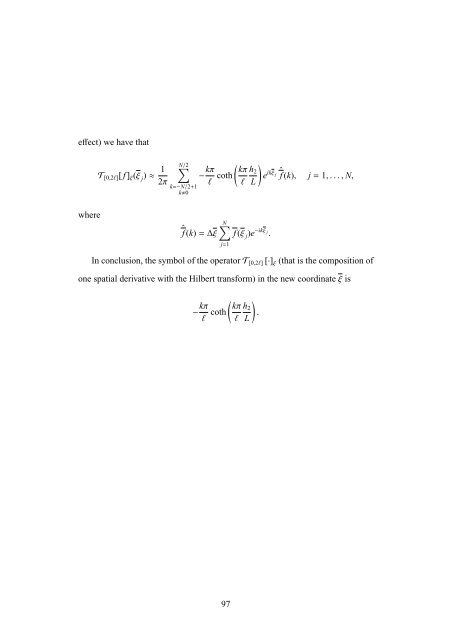
effect) we have that T [0,2l] [ f ] ξ (ξ j )≈ 1 2π ∑N/2 k=−N/2+1 k0 − kπ l coth ( kπ l ) h 2 e ikξ j ˆf (k), j=1,..., N, L where N∑ ˆf (k)=∆ξ f (ξ j )e −ikξ j . j=1 In conclusion, the symbol of the operatorT [0,2l] [·] ξ (that is the composition of one spatial derivative <strong>with</strong> the Hilbert trans<strong>for</strong>m) in the new coordinateξ is − kπ l coth ( kπ l ) h 2 . L 97
Bibliography [1] Artiles, W. & Nachbin, A., 2004. “Nonlinear evolution of surface gravity <strong>waves</strong> over highly variable depth,” Physical Review Letters, vol. 93, pp. 234501–1–234501–4. [2] Ascher, U. M. & Petzold, L. R., 1988. Computer Methods <strong>for</strong> Ordinary Differential Equations and Differential–Algebraic Equations, SIAM. [3] Benjamin, T. B., 1967. “Internal <strong>waves</strong> of permanent <strong>for</strong>m of great depth,” Journal of Fluid Mechanics, vol. 29, pp. 559–592. [4] Benjamin, T. B., Bona, J. L. & Mahony, J. J., 1972. “Model equations <strong>for</strong> long <strong>waves</strong> in nonlinear dispersive systems,” Philosophical Transactions of the Royal Society of London. Series A, Mathematical and Physical Sciences, vol. 272, No. 1220, pp. 47–78. [5] Camassa, R. & Levermore, C. D., 1997. “Layer-mean quantities, local conservation laws, and vorticity,” Physical Review Letters, vol. 78, pp. 650–653. [6] Choi, W., & Camassa, R., 1996. “Long <strong>internal</strong> <strong>waves</strong> of finite amplitude,” Physical Review Letters, vol. 77, pp. 1759–1762. 98
- Page 1 and 2:
INSTITUTO NACIONAL DE MATEMÁTICA P
- Page 3 and 4:
Acknowledgements First, I would lik
- Page 5 and 6:
4.1 Hierarchy of one-dimensional mo
- Page 7 and 8:
Resumo É obtido um modelo reduzido
- Page 9 and 10:
when the steepening of a given wave
- Page 11 and 12:
in particular that of solitary wave
- Page 13 and 14:
Chapter 2 Derivation of the reduced
- Page 15 and 16:
demands that η t + u i η x = w i
- Page 17 and 18:
function f (x, z, t), let its assoc
- Page 19 and 20:
Substitution of w 1 into Eq. (2.2)
- Page 21 and 22:
i. e. u 1z =βw 1x . Hence ( ) u (0
- Page 23 and 24:
fluid layer. 2.2 Connecting the upp
- Page 25 and 26:
Furthermore, [√ ( √ )] βφt x,
- Page 27 and 28:
The problem in conformal coordinate
- Page 29 and 30:
problem (2.22). Therefore, P x =−
- Page 31 and 32:
assumption was made on the wave amp
- Page 33 and 34:
Its linearization around the undist
- Page 35 and 36:
c 0 chosen, there will be a right-
- Page 37 and 38:
and for similar reasons η t +η x
- Page 39 and 40:
3. For system (2.28) a similar unid
- Page 41 and 42:
Chapter 3 A higher-order reduced mo
- Page 43 and 44:
expression above as Let us express
- Page 45 and 46:
and substituting in the asymptotic
- Page 47 and 48:
and it is easy to take x-derivative
- Page 49 and 50:
which together with η tt = ( (1−
- Page 51 and 52: For the weakly nonlinear model of o
- Page 53 and 54: Again, ω2 k 2 large. → 0 as k→
- Page 55 and 56: 2.6 2.4 2.2 ω/k 2 1.8 1.6 1.4 1.2
- Page 57 and 58: Chapter 4 Numerical results 4.1 Hie
- Page 59 and 60: Linear Weakly nonlinear Strongly no
- Page 61 and 62: is to approximate theξ-derivative
- Page 63 and 64: inary axis (where the eigenvalues o
- Page 65 and 66: 2.4 2.2 RK4 AM3 AM4 2 1.8 1.6 |R(z)
- Page 67 and 68: Also, recall that K1=E(η n , u n 1
- Page 69 and 70: • T is the convolution matrix for
- Page 71 and 72: The AM4 scheme used is: η n+1 j V
- Page 73 and 74: 0.6 0.4 0.2 η 0 −0.2 40 35 30 25
- Page 75 and 76: 0.6 0.5 0.4 0.3 η 0.2 0.1 0 −0.1
- Page 77 and 78: where c 1 and c 2 are two functions
- Page 79 and 80: 0.5 0.4 0.3 0.2 η 0.1 0 −0.1 −
- Page 81 and 82: 0.5 0.4 0.3 0.2 η 0.1 0 −0.1 −
- Page 83 and 84: 0.5 0.4 0.3 0.2 η 0.1 0 −0.1 −
- Page 85 and 86: 0.6 0.5 0.4 0.3 η 0.2 0.1 0 −0.1
- Page 87 and 88: 0.1 0.09 0.08 0.07 0.06 0.05 0.04 0
- Page 89 and 90: −η 0.1 0.08 0.06 0.04 0.02 0 60
- Page 91 and 92: Conclusions and future work In the
- Page 93 and 94: Appendix A Approximation for the ho
- Page 95 and 96: thenω 0 satisfies the Neumann prob
- Page 97 and 98: The inverseT ofT has a symbol−i t
- Page 99 and 100: Setξ=πξ/l. In the new coordinate
- Page 101: Takingξ-derivatives, φ ξ (ξ,ζ)
- Page 105 and 106: [16] Koop, C. G. & Butler, G., 1981