- Page 2:
This page intentionally left blank
- Page 8:
APPROACHES TO QUANTUM GRAVITY Towar
- Page 12:
A Sandra
- Page 18:
viii Contents 11 String theory, hol
- Page 22:
Contributors J. Ambjørn The Niels
- Page 26:
xii List of contributors D. Oriti M
- Page 32:
Preface Quantum Gravity is a dream,
- Page 36:
Preface xvii are following in their
- Page 40:
Preface xix enormous amount of prog
- Page 48:
1 Unfinished revolution C. ROVELLI
- Page 52:
Unfinished revolution 5 wit of empi
- Page 56:
Unfinished revolution 7 In general
- Page 60:
Unfinished revolution 9 However, re
- Page 64:
Unfinished revolution 11 References
- Page 68:
2 The fundamental nature of space a
- Page 72:
The fundamental nature of space and
- Page 76:
The fundamental nature of space and
- Page 80:
The fundamental nature of space and
- Page 84:
The fundamental nature of space and
- Page 88:
The fundamental nature of space and
- Page 92:
The fundamental nature of space and
- Page 96:
Does locality fail at intermediate
- Page 100:
Does locality fail at intermediate
- Page 104:
Does locality fail at intermediate
- Page 108:
Does locality fail at intermediate
- Page 112:
Does locality fail at intermediate
- Page 116:
∫ Does locality fail at intermedi
- Page 120:
Does locality fail at intermediate
- Page 124:
Does locality fail at intermediate
- Page 128:
Does locality fail at intermediate
- Page 132:
Prolegomena to any future Quantum G
- Page 136:
Prolegomena to any future Quantum G
- Page 140:
Prolegomena to any future Quantum G
- Page 144:
Prolegomena to any future Quantum G
- Page 148:
Prolegomena to any future Quantum G
- Page 152:
Prolegomena to any future Quantum G
- Page 156:
Prolegomena to any future Quantum G
- Page 160:
Prolegomena to any future Quantum G
- Page 164:
Prolegomena to any future Quantum G
- Page 168:
Prolegomena to any future Quantum G
- Page 172:
Prolegomena to any future Quantum G
- Page 176:
Prolegomena to any future Quantum G
- Page 180:
Spacetime symmetries in histories c
- Page 184:
Spacetime symmetries in histories c
- Page 188:
Spacetime symmetries in histories c
- Page 192:
Spacetime symmetries in histories c
- Page 196:
Spacetime symmetries in histories c
- Page 200:
Spacetime symmetries in histories c
- Page 204:
Spacetime symmetries in histories c
- Page 208:
Spacetime symmetries in histories c
- Page 212:
Categorical geometry and the mathem
- Page 216:
Categorical geometry and the mathem
- Page 220:
Categorical geometry and the mathem
- Page 224:
Categorical geometry and the mathem
- Page 228:
Categorical geometry and the mathem
- Page 232:
Categorical geometry and the mathem
- Page 236:
Categorical geometry and the mathem
- Page 240:
7 Emergent relativity O. DREYER 7.1
- Page 244:
A (a) Emergent relativity 101 (b) (
- Page 248:
Emergent relativity 103 It is here
- Page 252:
Emergent relativity 105 spacetime c
- Page 256:
Emergent relativity 107 φ A B Fig.
- Page 260:
Emergent relativity 109 If, on the
- Page 264:
8 Asymptotic safety R. PERCACCI 8.1
- Page 268:
Asymptotic safety 113 field and the
- Page 272:
Asymptotic safety 115 For example,
- Page 276:
Asymptotic safety 117 If we choose
- Page 280:
Asymptotic safety 119 complex field
- Page 284:
Asymptotic safety 121 2 G ~ ~ 1.5 1
- Page 288:
Asymptotic safety 123 larger, and i
- Page 292:
Asymptotic safety 125 Dimensional a
- Page 296:
Asymptotic safety 127 References [1
- Page 300:
9 New directions in background inde
- Page 304:
New directions in background indepe
- Page 308:
New directions in background indepe
- Page 312:
New directions in background indepe
- Page 316:
New directions in background indepe
- Page 320:
New directions in background indepe
- Page 324:
New directions in background indepe
- Page 328:
New directions in background indepe
- Page 332:
New directions in background indepe
- Page 336:
New directions in background indepe
- Page 340:
New directions in background indepe
- Page 344:
Questions and answers 151 Quantum G
- Page 348:
Questions and answers 153 was that
- Page 352:
Questions and answers 155 causality
- Page 356:
Questions and answers 157 to hold),
- Page 360:
Questions and answers 159 of how gr
- Page 364:
Questions and answers 161 the actio
- Page 368:
Questions and answers 163 allow us
- Page 372:
Questions and answers 165 - A-F.Mar
- Page 380:
10 Gauge/gravity duality G. HOROWIT
- Page 384:
Gauge/gravity duality 171 strong an
- Page 388:
Gauge/gravity duality 173 decompose
- Page 392:
Gauge/gravity duality 175 Here l s
- Page 396:
Gauge/gravity duality 177 There is
- Page 400:
Gauge/gravity duality 179 these are
- Page 404:
Gauge/gravity duality 181 leading t
- Page 408:
Gauge/gravity duality 183 states to
- Page 412:
Gauge/gravity duality 185 [6] N. Be
- Page 416:
11 String theory, holography and Qu
- Page 420:
String theory, holography and Quant
- Page 424:
String theory, holography and Quant
- Page 428:
String theory, holography and Quant
- Page 432:
String theory, holography and Quant
- Page 436:
String theory, holography and Quant
- Page 440:
String theory, holography and Quant
- Page 444:
String theory, holography and Quant
- Page 448:
String theory, holography and Quant
- Page 452:
String theory, holography and Quant
- Page 456:
String theory, holography and Quant
- Page 460:
String theory, holography and Quant
- Page 464:
String field theory 211 no tools to
- Page 468:
String field theory 213 made an ins
- Page 472:
(d) Cyclicity: ∫ ⋆= (−1) G G
- Page 476:
String field theory 217 however, th
- Page 480:
String field theory 219 12.2.3 Outs
- Page 484:
String field theory 221 a review) g
- Page 488:
String field theory 223 similar com
- Page 492:
String field theory 225 this; the p
- Page 496:
String field theory 227 [11] T. G.
- Page 500:
Questions and answers • Q - D. Or
- Page 504:
Questions and answers 231 condition
- Page 508:
Part III Loop quantum gravity and s
- Page 514:
236 T. Thiemann (anti)commute. We s
- Page 518:
238 T. Thiemann Notice that in gene
- Page 522:
240 T. Thiemann spectrum of all the
- Page 526:
242 T. Thiemann order to avoid anom
- Page 530:
244 T. Thiemann We consider spaceti
- Page 534:
246 T. Thiemann Hence both gauge gr
- Page 538:
248 T. Thiemann that Ĉ(N) cannot b
- Page 542:
250 T. Thiemann [8] R. Brunetti, K.
- Page 546:
252 T. Thiemann [48] M. Bojowald, H
- Page 550:
254 E. Livine SU(2) gauge theory. T
- Page 554:
256 E. Livine space; η IJ is the f
- Page 558:
258 E. Livine However, in contrast
- Page 562:
260 E. Livine (i) Either we work wi
- Page 566:
262 E. Livine At the end of the day
- Page 570:
264 E. Livine projector at the end
- Page 574:
266 E. Livine for a surface S inter
- Page 578:
268 E. Livine This constraint is sa
- Page 582:
270 E. Livine we do not need the se
- Page 586:
15 The spin foam representation of
- Page 590:
274 A. Perez in classical general r
- Page 594:
276 A. Perez where M = ×R (for an
- Page 598:
278 A. Perez the Levi-Civita tensor
- Page 602:
280 A. Perez k Tr[ k (W p )] ✄ j
- Page 606:
282 A. Perez j j j k j k m k m j j
- Page 610:
284 A. Perez Here we studied the in
- Page 614:
286 A. Perez A spin foam representa
- Page 618:
288 A. Perez master-constraint prog
- Page 622:
16 Three-dimensional spin foam Quan
- Page 626:
292 L. Freidel 16.3 The Ponzano-Reg
- Page 630:
294 L. Freidel under usual gauge tr
- Page 634:
296 L. Freidel is now constrained t
- Page 638:
298 L. Freidel 16.4.1 Mathematical
- Page 642:
300 L. Freidel Therefore, at first
- Page 646:
302 L. Freidel The inverse group Fo
- Page 650:
304 L. Freidel From this identity,
- Page 654:
306 L. Freidel choice of statistics
- Page 658:
308 L. Freidel A deeper study of th
- Page 662:
17 The group field theory approach
- Page 666:
312 D. Oriti simplicial complex, or
- Page 670:
314 D. Oriti are not all simultaneo
- Page 674:
316 D. Oriti diagrams correspond to
- Page 678:
318 D. Oriti is the simple fact tha
- Page 682:
320 D. Oriti better, by a single ma
- Page 686:
322 D. Oriti or SO(3, 1)) [8; 9; 10
- Page 690:
324 D. Oriti where: g i ∈ G, s i
- Page 694:
326 D. Oriti observables in GFTs ar
- Page 698:
328 D. Oriti research. On the other
- Page 702:
330 D. Oriti of the possibility of
- Page 706:
Questions and answers • Q - L. Cr
- Page 710:
334 Questions and answers I partly
- Page 714:
336 Questions and answers spectrum
- Page 720:
Part IV Discrete Quantum Gravity
- Page 726:
342 J. Ambjørn, J. Jurkiewicz and
- Page 730:
344 J. Ambjørn, J. Jurkiewicz and
- Page 734:
346 J. Ambjørn, J. Jurkiewicz and
- Page 738:
348 J. Ambjørn, J. Jurkiewicz and
- Page 742:
350 J. Ambjørn, J. Jurkiewicz and
- Page 746:
352 J. Ambjørn, J. Jurkiewicz and
- Page 750:
354 J. Ambjørn, J. Jurkiewicz and
- Page 754:
356 J. Ambjørn, J. Jurkiewicz and
- Page 758:
358 J. Ambjørn, J. Jurkiewicz and
- Page 762:
19 Quantum Regge calculus R. WILLIA
- Page 766:
362 R. Williams only in flat space
- Page 770:
364 R. Williams where V is the volu
- Page 774:
366 R. Williams equations of motion
- Page 778:
368 R. Williams Dropping the 1/d co
- Page 782:
370 R. Williams At a typical interi
- Page 786:
372 R. Williams about which it make
- Page 790:
374 R. Williams dealt with include
- Page 794:
376 R. Williams [27] H. W. Hamber,
- Page 798:
20 Consistent discretizations as a
- Page 802:
380 R. Gambini and J. Pullin The mo
- Page 806:
382 R. Gambini and J. Pullin phase
- Page 810:
384 R. Gambini and J. Pullin 2 1 q
- Page 814:
386 R. Gambini and J. Pullin of the
- Page 818:
388 R. Gambini and J. Pullin accept
- Page 822:
390 R. Gambini and J. Pullin isomor
- Page 826:
392 R. Gambini and J. Pullin [3] C.
- Page 830:
394 J. Henson all the other subject
- Page 834:
396 J. Henson z y x Fig. 21.1. A ca
- Page 838:
398 J. Henson this way, no discrete
- Page 842:
400 J. Henson out various sprinklin
- Page 846:
402 J. Henson commutes with rotatio
- Page 850:
404 J. Henson black hole entropy (o
- Page 854:
406 J. Henson “Kleitman-Rothschil
- Page 858:
408 J. Henson histories suggest any
- Page 862:
410 J. Henson the type normally use
- Page 866:
412 J. Henson [17] R. D. Sorkin (19
- Page 870:
Questions and answers • Q - J. He
- Page 874:
416 Questions and answers that the
- Page 878:
418 Questions and answers 2. The ab
- Page 882:
420 Questions and answers not unimp
- Page 886:
422 Questions and answers - A - R.
- Page 892:
Part V Effective models and Quantum
- Page 898:
428 G. Amelino-Camelia For this phe
- Page 902:
430 G. Amelino-Camelia correction t
- Page 906:
432 G. Amelino-Camelia to the fact
- Page 910:
434 G. Amelino-Camelia 22.2.2 Planc
- Page 914:
436 G. Amelino-Camelia formalism in
- Page 918:
438 G. Amelino-Camelia 22.3 On the
- Page 922:
440 G. Amelino-Camelia 22.4 Aside o
- Page 926:
442 G. Amelino-Camelia A theory wil
- Page 930:
444 G. Amelino-Camelia we might be
- Page 934:
446 G. Amelino-Camelia For the disp
- Page 938:
448 G. Amelino-Camelia References [
- Page 942:
23 Quantum Gravity and precision te
- Page 946:
452 C. Burgess with the following s
- Page 950:
454 C. Burgess For this reason it i
- Page 954:
456 C. Burgess ) E ( m ) P ( ( 1 2L
- Page 958:
458 C. Burgess the low-energy exper
- Page 962:
460 C. Burgess couplings contribute
- Page 966: 462 C. Burgess Non-relativistic sou
- Page 970: 464 C. Burgess contribute at any gi
- Page 974: 24 Algebraic approach to Quantum Gr
- Page 978: 468 S. Majid has been called a ‘P
- Page 982: 470 S. Majid α → u −1 αu + u
- Page 986: 472 S. Majid coordinates the coprod
- Page 990: 474 S. Majid Position Momentum Grav
- Page 994: 476 S. Majid quantum group acts cov
- Page 998: 478 S. Majid where we introduce p 0
- Page 1002: 480 S. Majid λ p 0 2 θ < 0 1.5 1
- Page 1006: 482 S. Majid to complete the struct
- Page 1010: 484 S. Majid C[SO 3,1 ]◮⊳U(R 3
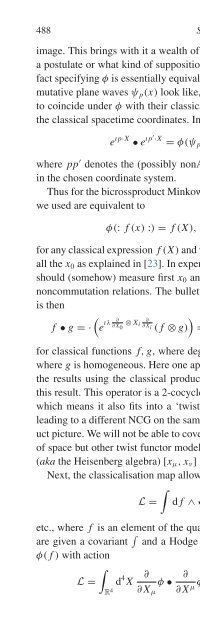
- Page 1014: 486 S. Majid 24.5 Physical interpre
- Page 1020: Algebraic approach to Quantum Gravi
- Page 1024: Algebraic approach to Quantum Gravi
- Page 1028: 25 Doubly special relativity J. KOW
- Page 1032: Doubly special relativity 495 DSR t
- Page 1036: Doubly special relativity 497 On th
- Page 1040: Doubly special relativity 499 some
- Page 1044: Doubly special relativity 501 [x 0
- Page 1048: Doubly special relativity 503 that
- Page 1052: Doubly special relativity 505 can b
- Page 1056: Doubly special relativity 507 scale
- Page 1060: 26 From quantum reference frames to
- Page 1064: From quantum reference frames to de
- Page 1068:
From quantum reference frames to de
- Page 1072:
From quantum reference frames to de
- Page 1076:
From quantum reference frames to de
- Page 1080:
From quantum reference frames to de
- Page 1084:
From quantum reference frames to de
- Page 1088:
From quantum reference frames to de
- Page 1092:
From quantum reference frames to de
- Page 1096:
From quantum reference frames to de
- Page 1100:
Lorentz invariance violation & its
- Page 1104:
Lorentz invariance violation & its
- Page 1108:
Lorentz invariance violation & its
- Page 1112:
Lorentz invariance violation & its
- Page 1116:
Lorentz invariance violation & its
- Page 1120:
Lorentz invariance violation & its
- Page 1124:
Lorentz invariance violation & its
- Page 1128:
Lorentz invariance violation & its
- Page 1132:
Lorentz invariance violation & its
- Page 1136:
Lorentz invariance violation & its
- Page 1140:
Generic predictions of quantum theo
- Page 1144:
Generic predictions of quantum theo
- Page 1148:
Generic predictions of quantum theo
- Page 1152:
Generic predictions of quantum theo
- Page 1156:
Generic predictions of quantum theo
- Page 1160:
Generic predictions of quantum theo
- Page 1164:
Generic predictions of quantum theo
- Page 1168:
Generic predictions of quantum theo
- Page 1172:
Generic predictions of quantum theo
- Page 1176:
Generic predictions of quantum theo
- Page 1180:
Generic predictions of quantum theo
- Page 1184:
Questions and answers • Q - L. Cr
- Page 1188:
Questions and answers 573 frame. Ju
- Page 1192:
Questions and answers 575 - A - J.
- Page 1196:
Questions and answers 577 where thi
- Page 1200:
Questions and answers 579 would all
- Page 1204:
Index 581 cosmology, 26, 155, 184,
- Page 1208:
Index 583 emergent, 99, 109, 163, 1


![arXiv:1001.0993v1 [hep-ph] 6 Jan 2010](https://img.yumpu.com/51282177/1/190x245/arxiv10010993v1-hep-ph-6-jan-2010.jpg?quality=85)


![arXiv:1008.3907v2 [astro-ph.CO] 1 Nov 2011](https://img.yumpu.com/48909562/1/190x245/arxiv10083907v2-astro-phco-1-nov-2011.jpg?quality=85)


![arXiv:1002.4928v1 [gr-qc] 26 Feb 2010](https://img.yumpu.com/41209516/1/190x245/arxiv10024928v1-gr-qc-26-feb-2010.jpg?quality=85)
![arXiv:1206.2653v1 [astro-ph.CO] 12 Jun 2012](https://img.yumpu.com/39510078/1/190x245/arxiv12062653v1-astro-phco-12-jun-2012.jpg?quality=85)
